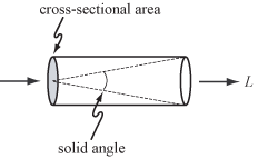
For geometric optics—i.e., to incoherent light and to objects larger than the wavelength of light—the fundamental carrier of light is a ray. The measure for the amount of light traveling along a ray is radiance, denoted by L and measured in W·sr⁻¹·m⁻², i.e., watts (W) per steradian (sr) per meter squared (m²). The steradian is a measure of solid angle, and meters squared are used as a measure of cross-sectional area, as shown at right.

The radiance along all such rays in a region of three-dimensional space illuminated by an unchanging arrangement of lights is called the plenoptic function.^[3] The plenoptic illumination function is an idealized function used in computer vision and computer graphics to express the image of a scene from any possible viewing position at any viewing angle at any point in time. It is not used in practice computationally, but is conceptually useful in understanding other concepts in vision and graphics.^[4] Since rays in space can be parameterized by three coordinates, x, y, and z and two angles θ and ϕ, as shown at left, it is a five-dimensional function, that is, a function over a five-dimensional manifold equivalent to the product of 3D Euclidean space and the 2-sphere.

The light field at each point in space can be treated as an infinite collection of vectors, one per direction impinging on the point, with lengths proportional to their radiances.

Integrating these vectors over any collection of lights, or over the entire sphere of directions, produces a single scalar value—the total irradiance at that point, and a resultant direction. The figure shows this calculation for the case of two light sources. In computer graphics, this vector-valued function of 3D space is called the vector irradiance field.^[6] The vector direction at each point in the field can be interpreted as the orientation of a flat surface placed at that point to most brightly illuminate it.

Higher dimensionality edit

Time, wavelength, and polarization angle can be treated as additional dimensions, yielding higher-dimensional functions, accordingly.

In a plenoptic function, if the region of interest contains a concave object (e.g., a cupped hand), then light leaving one point on the object may travel only a short distance before another point on the object blocks it. No practical device could measure the function in such a region.

However, for locations outside the object's convex hull (e.g., shrink-wrap), the plenoptic function can be measured by capturing multiple images. In this case the function contains redundant information, because the radiance along a ray remains constant throughout its length. The redundant information is exactly one dimension, leaving a four-dimensional function variously termed the photic field, the 4D light field^[7] or lumigraph.^[8] Formally, the field is defined as radiance along rays in empty space.

The set of rays in a light field can be parameterized in a variety of ways. The most common is the two-plane parameterization. While this parameterization cannot represent all rays, for example rays parallel to the two planes if the planes are parallel to each other, it relates closely to the analytic geometry of perspective imaging. A simple way to think about a two-plane light field is as a collection of perspective images of the st plane (and any objects that may lie astride or beyond it), each taken from an observer position on the uv plane. A light field parameterized this way is sometimes called a light slab.

Sound analog edit

The analog of the 4D light field for sound is the sound field or wave field, as in wave field synthesis, and the corresponding parametrization is the Kirchhoff–Helmholtz integral, which states that, in the absence of obstacles, a sound field over time is given by the pressure on a plane. Thus this is two dimensions of information at any point in time, and over time, a 3D field.

This two-dimensionality, compared with the apparent four-dimensionality of light, is because light travels in rays (0D at a point in time, 1D over time), while by the Huygens–Fresnel principle, a sound wave front can be modeled as spherical waves (2D at a point in time, 3D over time): light moves in a single direction (2D of information), while sound expands in every direction. However, light travelling in non-vacuous media may scatter in a similar fashion, and the irreversibility or information lost in the scattering is discernible in the apparent loss of a system dimension.

Because light field provides spatial and angular information, we can alter the position of focal planes after exposure, which is often termed refocusing. The principle of refocusing is to obtain conventional 2-D photographs from a light field through the integral transform. The transform takes a lightfield as its input and generates a photograph focused on a specific plane.

Assuming ${\displaystyle L_{F}(s,t,u,v)}$  represents a 4-D light field that records light rays traveling from position ${\displaystyle (u,v)}$  on the first plane to position ${\displaystyle (s,t)}$  on the second plane, where ${\displaystyle F}$  is the distance between two planes, a 2-D photograph at any depth ${\displaystyle \alpha F}$  can be obtained from the following integral transform:^[9]

${\displaystyle {\mathcal {P}}_{\alpha }\left[L_{F}\right](s,t)={1 \over \alpha ^{2}F^{2}}\iint L_{F}(u(1-1/\alpha )+s/\alpha ,v(1-1/\alpha )+t/\alpha ,u,v)~dudv}$ ,

or more concisely,

${\displaystyle {\mathcal {P}}_{\alpha }\left[L_{F}\right]({\boldsymbol {s}})={\frac {1}{\alpha ^{2}F^{2}}}\int L_{F}\left({\boldsymbol {u}}\left(1-{\frac {1}{\alpha }}\right)+{\frac {\boldsymbol {s}}{\alpha }},{\boldsymbol {u}}\right)d{\boldsymbol {u}}}$ ,

where ${\displaystyle {\boldsymbol {s}}=(s,t)}$ , ${\displaystyle {\boldsymbol {u}}=(u,v)}$ , and ${\displaystyle {\mathcal {P}}_{\alpha }\left[\cdot \right]}$  is the photography operator.

In practice, this formula cannot be directly used because a plenoptic camera usually captures discrete samples of the lightfield ${\displaystyle L_{F}(s,t,u,v)}$ , and hence resampling (or interpolation) is needed to compute ${\displaystyle L_{F}\left({\boldsymbol {u}}\left(1-{\frac {1}{\alpha }}\right)+{\frac {\boldsymbol {s}}{\alpha }},{\boldsymbol {u}}\right)}$ . Another problem is high computation complexity. To compute an ${\displaystyle N\times N}$  2-D photograph from an ${\displaystyle N\times N\times N\times N}$  4-D light field, the complexity of the formula is ${\displaystyle O(N^{4})}$ .^[9]

Fourier slice photography edit

One way to reduce the complexity of computation is to adopt the concept of Fourier slice theorem:^[9] The photography operator ${\displaystyle {\mathcal {P}}_{\alpha }\left[\cdot \right]}$  can be viewed as a shear followed by projection. The result should be proportional to a dilated 2-D slice of the 4-D Fourier transform of a light field. More precisely, a refocused image can be generated from the 4-D Fourier spectrum of a light field by extracting a 2-D slice, applying an inverse 2-D transform, and scaling. The asymptotic complexity of the algorithm is ${\displaystyle O(N^{2}\operatorname {log} N)}$ .

Discrete focal stack transform edit

Another way to efficiently compute 2-D photographs is to adopt discrete focal stack transform (DFST).^[10] DFST is designed to generate a collection of refocused 2-D photographs, or so-called Focal Stack. This method can be implemeted by fast fractional fourier transform (FrFT).

The discrete photography operator ${\displaystyle {\mathcal {P}}_{\alpha }\left[\cdot \right]}$  is defined as follows for a lightfield ${\displaystyle L_{F}({\boldsymbol {s}},{\boldsymbol {u}})}$  sampled in a 4-D grid ${\displaystyle {\boldsymbol {s}}=\Delta s{\tilde {\boldsymbol {s}}},{\tilde {\boldsymbol {s}}}=-{\boldsymbol {n}}_{\boldsymbol {s}},...,{\boldsymbol {n}}_{\boldsymbol {s}}}$ , ${\displaystyle {\boldsymbol {u}}=\Delta u{\tilde {\boldsymbol {u}}},{\tilde {\boldsymbol {u}}}=-{\boldsymbol {n}}_{\boldsymbol {u}},...,{\boldsymbol {n}}_{\boldsymbol {u}}}$ :

${\displaystyle {\mathcal {P}}_{q}[L]({\boldsymbol {s}})=\sum _{{\tilde {\boldsymbol {u}}}=-{\boldsymbol {n}}_{\boldsymbol {u}}}^{{\boldsymbol {n}}_{\boldsymbol {u}}}L({\boldsymbol {u}}q+{\boldsymbol {s}},{\boldsymbol {u}})\Delta {\boldsymbol {u}},\quad \Delta {\boldsymbol {u}}=\Delta u\Delta v,\quad q=\left(1-{\frac {1}{\alpha }}\right)}$ 

Because ${\displaystyle ({\boldsymbol {u}}q+{\boldsymbol {s}},{\boldsymbol {u}})}$  is usually not on the 4-D grid, DFST adopts trigonometric interpolation to compute the non-grid values.

The algorithm consists of these steps:

• Sample the light field ${\displaystyle L_{F}({\boldsymbol {s}},{\boldsymbol {u}})}$  with the sampling period ${\displaystyle \Delta s}$  and ${\displaystyle \Delta u}$  and get the discretized light field ${\displaystyle L_{F}^{d}({\boldsymbol {s}},{\boldsymbol {u}})}$ .
• Pad ${\displaystyle L_{F}^{d}({\boldsymbol {s}},{\boldsymbol {u}})}$  with zeros such that the signal length is enough for FrFT without aliasing.
• For every ${\displaystyle {\boldsymbol {u}}}$ , compute the Discrete Fourier transform of ${\displaystyle L_{F}^{d}({\boldsymbol {s}},{\boldsymbol {u}})}$ , and get the result ${\displaystyle R1}$ .
• For every focal length ${\displaystyle \alpha F}$ , compute the fractional fourier transform of ${\displaystyle R1}$ , where the order of the transform depends on ${\displaystyle \alpha }$ , and get the result ${\displaystyle R2}$ .
• Compute the inverse Discrete Fourier transform of ${\displaystyle R2}$ .
• Remove the marginal pixels of ${\displaystyle R2}$  so that each 2-D photograph has the size ${\displaystyle (2{n}_{\boldsymbol {s}}+1)\times (2{n}_{\boldsymbol {s}}+1)}$ 

In computer graphics, light fields are typically produced either by rendering a 3D model or by photographing a real scene. In either case, to produce a light field, views must be obtained for a large collection of viewpoints. Depending on the parameterization, this collection typically spans some portion of a line, circle, plane, sphere, or other shape, although unstructured collections are possible.^[11]

Devices for capturing light fields photographically may include a moving handheld camera or a robotically controlled camera,^[12] an arc of cameras (as in the bullet time effect used in The Matrix), a dense array of cameras,^[13] handheld cameras,^[14][15] microscopes,^[16] or other optical system.^[17]

The number of images in a light field depends on the application. A light field capture of Michelangelo's statue of Night^[18] contains 24,000 1.3-megapixel images, which is considered large as of 2022. For light field rendering to completely capture an opaque object, images must be taken of at least the front and back. Less obviously, for an object that lies astride the st plane, finely spaced images must be taken on the uv plane (in the two-plane parameterization shown above).

The number and arrangement of images in a light field, and the resolution of each image, are together called the "sampling" of the 4D light field.^[19] Also of interest are the effects of occlusion,^[20] lighting and reflection.^[21]

Illumination engineering edit

Gershun's reason for studying the light field was to derive (in closed form) illumination patterns that would be observed on surfaces due to light sources of various shapes positioned above these surface.^[23] The branch of optics devoted to illumination engineering is nonimaging optics.^[24] It extensively uses the concept of flow lines (Gershun's flux lines) and vector flux (Gershun's light vector). However, the light field (in this case the positions and directions defining the light rays) is commonly described in terms of phase space and Hamiltonian optics.

Light field rendering edit

Extracting appropriate 2D slices from the 4D light field of a scene, enables novel views of the scene.^[25] Depending on the parameterization of the light field and slices, these views might be perspective, orthographic, crossed-slit,^[26] general linear cameras,^[27] multi-perspective,^[28] or another type of projection. Light field rendering is one form of image-based rendering.

Synthetic aperture photography edit

Integrating an appropriate 4D subset of the samples in a light field can approximate the view that would be captured by a camera having a finite (i.e., non-pinhole) aperture. Such a view has a finite depth of field. Shearing or warping the light field before performing this integration can focus on different fronto-parallel^[29] or oblique^[30] planes. Images captured by digital cameras that capture the light field^[14] can be refocused.

3D display edit

Presenting a light field using technology that maps each sample to the appropriate ray in physical space produces an autostereoscopic visual effect akin to viewing the original scene. Non-digital technologies for doing this include integral photography, parallax panoramagrams, and holography; digital technologies include placing an array of lenslets over a high-resolution display screen, or projecting the imagery onto an array of lenslets using an array of video projectors. An array of video cameras can capture and display a time-varying light field. This essentially constitutes a 3D television system.^[31] Modern approaches to light-field display explore co-designs of optical elements and compressive computation to achieve higher resolutions, increased contrast, wider fields of view, and other benefits.^[32]

Brain imaging edit

Neural activity can be recorded optically by genetically encoding neurons with reversible fluorescent markers such as GCaMP that indicate the presence of calcium ions in real time. Since light field microscopy captures full volume information in a single frame, it is possible to monitor neural activity in individual neurons randomly distributed in a large volume at video framerate.^[33] Quantitative measurement of neural activity can be done despite optical aberrations in brain tissue and without reconstructing a volume image,^[34] and be used to monitor activity in thousands of neurons.^[35]

Generalized Scene Reconstruction (GSR) edit

This is a method of 3D reconstruction from multiple images that creates a scene model comprising a generalized light field and a relightable matter field.^[36] The generalized light field represents light flowing in every direction through every point in the field. The relightable matter field represents the light interaction properties and emissivity of matter occupying every point in the field. Scene data structures can be implemented using Neural Networks,^[37][38][39] and Physics-based structures,^[40][41] among others.^[36] The light and matter fields are at least partially disentangled.^[36][42]

Holographic stereograms edit

Image generation and predistortion of synthetic imagery for holographic stereograms is one of the earliest examples of computed light fields.^[43]

Glare reduction edit

Glare arises due to multiple scattering of light inside the camera body and lens optics that reduces image contrast. While glare has been analyzed in 2D image space,^[44] it is useful to identify it as a 4D ray-space phenomenon.^[45] Statistically analyzing the ray-space inside a camera allows the classification and removal of glare artifacts. In ray-space, glare behaves as high frequency noise and can be reduced by outlier rejection. Such analysis can be performed by capturing the light field inside the camera, but it results in the loss of spatial resolution. Uniform and non-uniform ray sampling can be used to reduce glare without significantly compromising image resolution.^[45]

• Angle–sensitive pixel
• Dual photography
• Light-field camera
• Lytro
• Raytrix
• Reflectance paper

Theory edit

• Adelson, E.H., Bergen, J.R. (1991). "The Plenoptic Function and the Elements of Early Vision", In Computation Models of Visual Processing, M. Landy and J.A. Movshon, eds., MIT Press, Cambridge, 1991, pp. 3–20.
• Arvo, J. (1994). "The Irradiance Jacobian for Partially Occluded Polyhedral Sources", Proc. ACM SIGGRAPH, ACM Press, pp. 335–342.
• Bolles, R.C., Baker, H. H., Marimont, D.H. (1987). "Epipolar-Plane Image Analysis: An Approach to Determining Structure from Motion", International Journal of Computer Vision, Vol. 1, No. 1, 1987, Kluwer Academic Publishers, pp 7–55.
• Faraday, M., "Thoughts on Ray Vibrations", Philosophical Magazine, S.3, Vol XXVIII, N188, May 1846.
• Gershun, A. (1936). "The Light Field", Moscow, 1936. Translated by P. Moon and G. Timoshenko in Journal of Mathematics and Physics, Vol. XVIII, MIT, 1939, pp. 51–151.
• Gortler, S.J., Grzeszczuk, R., Szeliski, R., Cohen, M. (1996). "The Lumigraph", Proc. ACM SIGGRAPH, ACM Press, pp. 43–54.
• Levoy, M., Hanrahan, P. (1996). "Light Field Rendering", Proc. ACM SIGGRAPH, ACM Press, pp. 31–42.
• Moon, P., Spencer, D.E. (1981). The Photic Field, MIT Press.
• Wong, T.T., Fu, C.W., Heng, P.A., Leung C.S. (2002). "The Plenoptic-Illumination Function", IEEE Trans. Multimedia, Vol. 4, No. 3, pp. 361–371.

Analysis edit

• G. Wetzstein, I. Ihrke, W. Heidrich (2013) "On Plenoptic Multiplexing and Reconstruction", International Journal of Computer Vision (IJCV), Volume 101, Issue 2, pp. 384–400.
• Ramamoorthi, R., Mahajan, D., Belhumeur, P. (2006). "A First Order Analysis of Lighting, Shading, and Shadows", ACM TOG.
• Zwicker, M., Matusik, W., Durand, F., Pfister, H. (2006). "Antialiasing for Automultiscopic 3D Displays", Eurographics Symposium on Rendering, 2006.
• Ng, R. (2005). "Fourier Slice Photography", Proc. ACM SIGGRAPH, ACM Press, pp. 735–744.
• Durand, F., Holzschuch, N., Soler, C., Chan, E., Sillion, F. X. (2005). "A Frequency Analysis of Light Transport", Proc. ACM SIGGRAPH, ACM Press, pp. 1115–1126.
• Chai, J.-X., Tong, X., Chan, S.-C., Shum, H. (2000). "Plenoptic Sampling", Proc. ACM SIGGRAPH, ACM Press, pp. 307–318.
• Halle, M. (1994) "Holographic Stereograms as Discrete imaging systems"^{[permanent dead link]}, in SPIE Proc. Vol. #2176: Practical Holography VIII, S.A. Benton, ed., pp. 73–84.
• Yu, J., McMillan, L. (2004). "General Linear Cameras", Proc. ECCV 2004, Lecture Notes in Computer Science, pp. 14–27.

Cameras edit

• Marwah, K., Wetzstein, G., Bando, Y., Raskar, R. (2013). "Compressive Light Field Photography using Overcomplete Dictionaries and Optimized Projections", ACM Transactions on Graphics (SIGGRAPH).
• Liang, C.K., Lin, T.H., Wong, B.Y., Liu, C., Chen, H. H. (2008). "Programmable Aperture Photography:Multiplexed Light Field Acquisition", Proc. ACM SIGGRAPH.
• Veeraraghavan, A., Raskar, R., Agrawal, A., Mohan, A., Tumblin, J. (2007). "Dappled Photography: Mask Enhanced Cameras for Heterodyned Light Fields and Coded Aperture Refocusing", Proc. ACM SIGGRAPH.
• Georgiev, T., Zheng, C., Nayar, S., Curless, B., Salesin, D., Intwala, C. (2006). "Spatio-angular Resolution Trade-offs in Integral Photography", Proc. EGSR 2006.
• Kanade, T., Saito, H., Vedula, S. (1998). "The 3D Room: Digitizing Time-Varying 3D Events by Synchronized Multiple Video Streams", Tech report CMU-RI-TR-98-34, December 1998.
• Levoy, M. (2002). Stanford Spherical Gantry.
• Levoy, M., Ng, R., Adams, A., Footer, M., Horowitz, M. (2006). "Light Field Microscopy", ACM Transactions on Graphics (Proc. SIGGRAPH), Vol. 25, No. 3.
• Ng, R., Levoy, M., Brédif, M., Duval, G., Horowitz, M., Hanrahan, P. (2005). "Light Field Photography with a Hand-Held Plenoptic Camera", Stanford Tech Report CTSR 2005–02, April, 2005.
• Wilburn, B., Joshi, N., Vaish, V., Talvala, E., Antunez, E., Barth, A., Adams, A., Levoy, M., Horowitz, M. (2005). "High Performance Imaging Using Large Camera Arrays", ACM Transactions on Graphics (Proc. SIGGRAPH), Vol. 24, No. 3, pp. 765–776.
• Yang, J.C., Everett, M., Buehler, C., McMillan, L. (2002). "A Real-Time Distributed Light Field Camera", Proc. Eurographics Rendering Workshop 2002.
• "The CAFADIS camera"

Displays edit

• Wetzstein, G., Lanman, D., Hirsch, M., Raskar, R. (2012). "Tensor Displays: Compressive Light Field Display using Multilayer Displays with Directional Backlighting", ACM Transactions on Graphics (SIGGRAPH)
• Wetzstein, G., Lanman, D., Heidrich, W., Raskar, R. (2011). "Layered 3D: Tomographic Image Synthesis for Attenuation-based Light Field and High Dynamic Range Displays", ACM Transactions on Graphics (SIGGRAPH)
• Lanman, D., Wetzstein, G., Hirsch, M., Heidrich, W., Raskar, R. (2011). "Polarization Fields: Dynamic Light Field Display using Multi-Layer LCDs", ACM Transactions on Graphics (SIGGRAPH Asia)
• Lanman, D., Hirsch, M. Kim, Y., Raskar, R. (2010). "HR3D: Glasses-free 3D Display using Dual-stacked LCDs High-Rank 3D Display using Content-Adaptive Parallax Barriers", ACM Transactions on Graphics (SIGGRAPH Asia)
• Matusik, W., Pfister, H. (2004). "3D TV: A Scalable System for Real-Time Acquisition, Transmission, and Autostereoscopic Display of Dynamic Scenes", Proc. ACM SIGGRAPH, ACM Press.
• Javidi, B., Okano, F., eds. (2002). Three-Dimensional Television, Video and Display Technologies, Springer-Verlag.
• Klug, M., Burnett, T., Fancello, A., Heath, A., Gardner, K., O'Connell, S., Newswanger, C. (2013). "A Scalable, Collaborative, Interactive Light-field Display System", SID Symposium Digest of Technical Papers
• Fattal, D., Peng, Z., Tran, T., Vo, S., Fiorentino, M., Brug, J., Beausoleil, R. (2013). "A multi-directional backlight for a wide-angle, glasses-free three-dimensional display", Nature 495, 348–351

Archives edit

• "The Stanford Light Field Archive"
• "UCSD/MERL Light Field Repository"
• "The HCI Light Field Benchmark"
• "Synthetic Light Field Archive"

Applications edit

• Grosenick, L., Anderson, T., Smith S. J. (2009) "Elastic Source Selection for in vivo imaging of neuronal ensembles." From Nano to Macro, 6th IEEE International Symposium on Biomedical Imaging. (2009) 1263–1266.
• Grosenick, L., Broxton, M., Kim, C. K., Liston, C., Poole, B., Yang, S., Andalman, A., Scharff, E., Cohen, N., Yizhar, O., Ramakrishnan, C., Ganguli, S., Suppes, P., Levoy, M., Deisseroth, K. (2017) "Identification of cellular-activity dynamics across large tissue volumes in the mammalian brain" bioRxiv 132688; doi: Identification of cellular-activity dynamics across large tissue volumes in the mammalian brain.
• Heide, F., Wetzstein, G., Raskar, R., Heidrich, W. (2013) "Adaptive Image Synthesis for Compressive Displays", ACM Transactions on Graphics (SIGGRAPH)
• Wetzstein, G., Raskar, R., Heidrich, W. (2011) "Hand-Held Schlieren Photography with Light Field Probes", IEEE International Conference on Computational Photography (ICCP)
• Pérez, F., Marichal, J. G., Rodriguez, J.M. (2008). "The Discrete Focal Stack Transform", Proc. EUSIPCO
• Raskar, R., Agrawal, A., Wilson, C., Veeraraghavan, A. (2008). "Glare Aware Photography: 4D Ray Sampling for Reducing Glare Effects of Camera Lenses", Proc. ACM SIGGRAPH.
• Talvala, E-V., Adams, A., Horowitz, M., Levoy, M. (2007). "Veiling Glare in High Dynamic Range Imaging", Proc. ACM SIGGRAPH.
• Halle, M., Benton, S., Klug, M., Underkoffler, J. (1991). "The UltraGram: A Generalized Holographic Stereogram"^{[permanent dead link]}, SPIE Vol. 1461, Practical Holography V, S.A. Benton, ed., pp. 142–155.
• Zomet, A., Feldman, D., Peleg, S., Weinshall, D. (2003). "Mosaicing New Views: The Crossed-Slits Projection", IEEE Transactions on Pattern Analysis and Machine Intelligence (PAMI), Vol. 25, No. 6, June 2003, pp. 741–754.
• Vaish, V., Garg, G., Talvala, E., Antunez, E., Wilburn, B., Horowitz, M., Levoy, M. (2005). "Synthetic Aperture Focusing using a Shear-Warp Factorization of the Viewing Transform", Proc. Workshop on Advanced 3D Imaging for Safety and Security, in conjunction with CVPR 2005.
• Bedard, N., Shope, T., Hoberman, A., Haralam, M. A., Shaikh, N., Kovačević, J., Balram, N., Tošić, I. (2016). "Light field otoscope design for 3D in vivo imaging of the middle ear". Biomedical optics express, 8(1), pp. 260–272.
• Karygianni, S., Martinello, M., Spinoulas, L., Frossard, P., Tosic, I. (2018). "Automated eardrum registration from light-field data". IEEE International Conference on Image Processing (ICIP)
• Rademacher, P., Bishop, G. (1998). "Multiple-Center-of-Projection Images", Proc. ACM SIGGRAPH, ACM Press.
• Isaksen, A., McMillan, L., Gortler, S.J. (2000). "Dynamically Reparameterized Light Fields", Proc. ACM SIGGRAPH, ACM Press, pp. 297–306.
• Buehler, C., Bosse, M., McMillan, L., Gortler, S., Cohen, M. (2001). "Unstructured Lumigraph Rendering", Proc. ACM SIGGRAPH, ACM Press.
• Ashdown, I. (1993). "Near-Field Photometry: A New Approach", Journal of the Illuminating Engineering Society, Vol. 22, No. 1, Winter, 1993, pp. 163–180.
• Chaves, J. (2015) "Introduction to Nonimaging Optics, Second Edition", CRC Press
• Winston, R., Miñano, J.C., Benitez, P.G., Shatz, N., Bortz, J.C., (2005) "Nonimaging Optics", Academic Press
• Pégard, N. C., Liu H.Y., Antipa, N., Gerlock M., Adesnik, H., and Waller, L.. Compressive light-field microscopy for 3D neural activity recording. Optica 3, no. 5, pp. 517–524 (2016).
• Leffingwell, J., Meagher, D., Mahmud, K., Ackerson, S. (2018). "Generalized Scene Reconstruction." arXiv:1803.08496v3 [cs.CV], pp. 1–13.
• Mildenhall, B., Srinivasan, P. P., Tancik, M., Barron, J. T., Ramamoorthi, R., & Ng, R. (2020). “NeRF: Representing scenes as neural radiance fields for view synthesis.” Computer Vision – ECCV 2020, 405–421.
• Yu, A., Fridovich-Keil, S., Tancik, M., Chen, Q., Recht, B., Kanazawa, A. (2021). "Plenoxels: Radiance Fields without Neural Networks." arXiv:2111.11215, pp. 1–25
• Perez, CC; Lauri, A; et al. (September 2015). "Calcium neuroimaging in behaving zebrafish larvae using a turn-key light field camera". Journal of Biomedical Optics. 20 (9): 096009. Bibcode:2015JBO....20i6009C. doi:10.1117/1.JBO.20.9.096009. PMID 26358822.
• Perez, C. C., Lauri, A., Symvoulidis, P., Cappetta, M., Erdmann, A., & Westmeyer, G. G. (2015). Calcium neuroimaging in behaving zebrafish larvae using a turn-key light field camera. Journal of Biomedical Optics, 20(9), 096009-096009.
• León, K., Galvis, L., and Arguello, H. (2016). "Reconstruction of multispectral light field (5d plenoptic function) based on compressive sensing with colored coded apertures from 2D projections" Revista Facultad de Ingeniería Universidad de Antioquia 80, pp. 131.