


Summary
In theoretical physics and mathematical physics, analytical mechanics, or theoretical mechanics is a collection of closely related formulations of classical mechanics. Analytical mechanics uses scalar properties of motion representing the system as a whole—usually its kinetic energy and potential energy. The equations of motion are derived from the scalar quantity by some underlying principle about the scalar's variation.
Analytical mechanics was developed by many scientists and mathematicians during the 18th century and onward, after Newtonian mechanics. Newtonian mechanics considers vector quantities of motion, particularly accelerations, momenta, forces, of the constituents of the system; it can also be called vectorial mechanics.[1] A scalar is a quantity, whereas a vector is represented by quantity and direction. The results of these two different approaches are equivalent, but the analytical mechanics approach has many advantages for complex problems.
Analytical mechanics takes advantage of a system's constraints to solve problems. The constraints limit the degrees of freedom the system can have, and can be used to reduce the number of coordinates needed to solve for the motion. The formalism is well suited to arbitrary choices of coordinates, known in the context as generalized coordinates. The kinetic and potential energies of the system are expressed using these generalized coordinates or momenta, and the equations of motion can be readily set up, thus analytical mechanics allows numerous mechanical problems to be solved with greater efficiency than fully vectorial methods. It does not always work for non-conservative forces or dissipative forces like friction, in which case one may revert to Newtonian mechanics.
Two dominant branches of analytical mechanics are Lagrangian mechanics (using generalized coordinates and corresponding generalized velocities in configuration space) and Hamiltonian mechanics (using coordinates and corresponding momenta in phase space). Both formulations are equivalent by a Legendre transformation on the generalized coordinates, velocities and momenta; therefore, both contain the same information for describing the dynamics of a system. There are other formulations such as Hamilton–Jacobi theory, Routhian mechanics, and Appell's equation of motion. All equations of motion for particles and fields, in any formalism, can be derived from the widely applicable result called the principle of least action. One result is Noether's theorem, a statement which connects conservation laws to their associated symmetries.
Analytical mechanics does not introduce new physics and is not more general than Newtonian mechanics. Rather it is a collection of equivalent formalisms which have broad application. In fact the same principles and formalisms can be used in relativistic mechanics and general relativity, and with some modifications, quantum mechanics and quantum field theory.
Analytical mechanics is used widely, from fundamental physics to applied mathematics, particularly chaos theory.
The methods of analytical mechanics apply to discrete particles, each with a finite number of degrees of freedom. They can be modified to describe continuous fields or fluids, which have infinite degrees of freedom. The definitions and equations have a close analogy with those of mechanics.
Motivation for analytical mechanics edit
The goal of mechanical theory is to solve mechanical problems, such as arise in physics and engineering. Starting from a physical system—such as a mechanism or a star system—a mathematical model is developed in the form of a differential equation. The model can be solved numerically or analytically to determine the motion of the system.
Newton's vectorial approach to mechanics describes motion with the help of vector quantities such as force, velocity, acceleration. These quantities characterise the motion of a body idealised as a "mass point" or a "particle" understood as a single point to which a mass is attached. Newton's method has been successfully applied to a wide range of physical problems, including the motion of a particle in Earth's gravitational field and the motion of planets around the Sun. In this approach, Newton's laws describe the motion by a differential equation and then the problem is reduced to the solving of that equation.
When a mechanical system contains many particles, however (such as a complex mechanism or a fluid), Newton's approach is difficult to apply. Using a Newtonian approach is possible, under proper precautions, namely isolating each single particle from the others, and determining all the forces acting on it. Such analysis is cumbersome even in relatively simple systems. Newton thought that his third law "action equals reaction" would take care of all complications.[citation needed] This is false even for such simple system as rotations of a solid body.[clarification needed] In more complicated systems, the vectorial approach cannot give an adequate description.
The analytical approach simplifies problems by treating mechanical systems as ensembles of particles that interact with each other, rather considering each particle as an isolated unit. In the vectorial approach, forces must be determined individually for each particle, whereas in the analytical approach it is enough to know one single function which contains implicitly all the forces acting on and in the system. Such simplification is often done using certain kinematic conditions which are stated a priori. However, the analytical treatment does not require the knowledge of these forces and takes these kinematic conditions for granted.[citation needed]
Still, deriving the equations of motion of a complicated mechanical system requires a unifying basis from which they follow.[clarification needed] This is provided by various variational principles: behind each set of equations there is a principle that expresses the meaning of the entire set. Given a fundamental and universal quantity called action, the principle that this action be stationary under small variation of some other mechanical quantity generates the required set of differential equations. The statement of the principle does not require any special coordinate system, and all results are expressed in generalized coordinates. This means that the analytical equations of motion do not change upon a coordinate transformation, an invariance property that is lacking in the vectorial equations of motion.[2]
It is not altogether clear what is meant by 'solving' a set of differential equations. A problem is regarded as solved when the particles coordinates at time t are expressed as simple functions of t and of parameters defining the initial positions and velocities. However, 'simple function' is not a well-defined concept: nowadays, a function f(t) is not regarded as a formal expression in t (elementary function) as in the time of Newton but most generally as a quantity determined by t, and it is not possible to draw a sharp line between 'simple' and 'not simple' functions. If one speaks merely of 'functions', then every mechanical problem is solved as soon as it has been well stated in differential equations, because given the initial conditions and t determine the coordinates at t. This is a fact especially at present with the modern methods of computer modelling which provide arithmetical solutions to mechanical problems to any desired degree of accuracy, the differential equations being replaced by difference equations.
Still, though lacking precise definitions, it is obvious that the two-body problem has a simple solution, whereas the three-body problem has not. The two-body problem is solved by formulas involving parameters; their values can be changed to study the class of all solutions, that is, the mathematical structure of the problem. Moreover, an accurate mental or drawn picture can be made for the motion of two bodies, and it can be as real and accurate as the real bodies moving and interacting. In the three-body problem, parameters can also be assigned specific values; however, the solution at these assigned values or a collection of such solutions does not reveal the mathematical structure of the problem. As in many other problems, the mathematical structure can be elucidated only by examining the differential equations themselves.
Analytical mechanics aims at even more: not at understanding the mathematical structure of a single mechanical problem, but that of a class of problems so wide that they encompass most of mechanics. It concentrates on systems to which Lagrangian or Hamiltonian equations of motion are applicable and that include a very wide range of problems indeed.[3]
Development of analytical mechanics has two objectives: (i) increase the range of solvable problems by developing standard techniques with a wide range of applicability, and (ii) understand the mathematical structure of mechanics. In the long run, however, (ii) can help (i) more than a concentration on specific problems for which methods have already been designed.
Intrinsic motion edit
Generalized coordinates and constraints edit
In Newtonian mechanics, one customarily uses all three Cartesian coordinates, or other 3D coordinate system, to refer to a body's position during its motion. In physical systems, however, some structure or other system usually constrains the body's motion from taking certain directions and pathways. So a full set of Cartesian coordinates is often unneeded, as the constraints determine the evolving relations among the coordinates, which relations can be modeled by equations corresponding to the constraints. In the Lagrangian and Hamiltonian formalisms, the constraints are incorporated into the motion's geometry, reducing the number of coordinates to the minimum needed to model the motion. These are known as generalized coordinates, denoted qi (i = 1, 2, 3...).[4]: 231
Difference between curvillinear and generalized coordinates edit
Generalized coordinates incorporate constraints on the system. There is one generalized coordinate qi for each degree of freedom (for convenience labelled by an index i = 1, 2...N), i.e. each way the system can change its configuration; as curvilinear lengths or angles of rotation. Generalized coordinates are not the same as curvilinear coordinates. The number of curvilinear coordinates equals the dimension of the position space in question (usually 3 for 3d space), while the number of generalized coordinates is not necessarily equal to this dimension; constraints can reduce the number of degrees of freedom (hence the number of generalized coordinates required to define the configuration of the system), following the general rule:[5][dubious ]
For a system with N degrees of freedom, the generalized coordinates can be collected into an N-tuple:


D'Alembert's principle of virtual work edit
D'Alembert's principle states that infinitesimal virtual work done by a force across reversible displacements is zero, which is the work done by a force consistent with ideal constraints of the system. The idea of a constraint is useful – since this limits what the system can do, and can provide steps to solving for the motion of the system. The equation for D'Alembert's principle is:[6]: 265


where T is the total kinetic energy of the system, and the notation

Constraints edit
If the curvilinear coordinate system is defined by the standard position vector r, and if the position vector can be written in terms of the generalized coordinates q and time t in the form:

Lagrangian mechanics edit
The introduction of generalized coordinates and the fundamental Lagrangian function:

where T is the total kinetic energy and V is the total potential energy of the entire system, then either following the calculus of variations or using the above formula – lead to the Euler–Lagrange equations;

which are a set of N second-order ordinary differential equations, one for each qi(t).
This formulation identifies the actual path followed by the motion as a selection of the path over which the time integral of kinetic energy is least, assuming the total energy to be fixed, and imposing no conditions on the time of transit.
The Lagrangian formulation uses the configuration space of the system, the set of all possible generalized coordinates:

where is N-dimensional real space (see also set-builder notation). The particular solution to the Euler–Lagrange equations is called a (configuration) path or trajectory, i.e. one particular q(t) subject to the required initial conditions. The general solutions form a set of possible configurations as functions of time:


The configuration space can be defined more generally, and indeed more deeply, in terms of topological manifolds and the tangent bundle.
Hamiltonian mechanics edit
The Legendre transformation of the Lagrangian replaces the generalized coordinates and velocities (q, q̇) with (q, p); the generalized coordinates and the generalized momenta conjugate to the generalized coordinates:

and introduces the Hamiltonian (which is in terms of generalized coordinates and momenta):

where denotes the dot product, also leading to Hamilton's equations:


which are now a set of 2N first-order ordinary differential equations, one for each qi(t) and pi(t). Another result from the Legendre transformation relates the time derivatives of the Lagrangian and Hamiltonian:

which is often considered one of Hamilton's equations of motion additionally to the others. The generalized momenta can be written in terms of the generalized forces in the same way as Newton's second law:

Analogous to the configuration space, the set of all momenta is the generalized momentum space:

("Momentum space" also refers to "k-space"; the set of all wave vectors (given by De Broglie relations) as used in quantum mechanics and theory of waves)
The set of all positions and momenta form the phase space:

that is, the Cartesian product of the configuration space and generalized momentum space.
A particular solution to Hamilton's equations is called a phase path, a particular curve (q(t),p(t)) subject to the required initial conditions. The set of all phase paths, the general solution to the differential equations, is the phase portrait:

The Poisson bracket edit
All dynamical variables can be derived from position q, momentum p, and time t, and written as a function of these: A = A(q, p, t). If A(q, p, t) and B(q, p, t) are two scalar valued dynamical variables, the Poisson bracket is defined by the generalized coordinates and momenta:

Calculating the total derivative of one of these, say A, and substituting Hamilton's equations into the result leads to the time evolution of A:

This equation in A is closely related to the equation of motion in the Heisenberg picture of quantum mechanics, in which classical dynamical variables become quantum operators (indicated by hats (^)), and the Poisson bracket is replaced by the commutator of operators via Dirac's canonical quantization:
![{\displaystyle \{A,B\}\rightarrow {\frac {1}{i\hbar }}[{\hat {A}},{\hat {B}}]\,.}](https://wikimedia.org/api/rest_v1/media/math/render/svg/0990f0c0d756e9d159c393f67053ba88f848789e)
Properties of the Lagrangian and the Hamiltonian edit
Following are overlapping properties between the Lagrangian and Hamiltonian functions.[5][8]
- All the individual generalized coordinates qi(t), velocities q̇i(t) and momenta pi(t) for every degree of freedom are mutually independent. Explicit time-dependence of a function means the function actually includes time t as a variable in addition to the q(t), p(t), not simply as a parameter through q(t) and p(t), which would mean explicit time-independence.
- The Lagrangian is invariant under addition of the total time derivative of any function of q' and t, that is: so each Lagrangian L and L describe exactly the same motion. In other words, the Lagrangian of a system is not unique.
- Analogously, the Hamiltonian is invariant under addition of the partial time derivative of any function of q, p and t, that is: (K is a frequently used letter in this case). This property is used in canonical transformations (see below).
- If the Lagrangian is independent of some generalized coordinates, then the generalized momenta conjugate to those coordinates are constants of the motion, i.e. are conserved, this immediately follows from Lagrange's equations: Such coordinates are "cyclic" or "ignorable". It can be shown that the Hamiltonian is also cyclic in exactly the same generalized coordinates.
- If the Lagrangian is time-independent the Hamiltonian is also time-independent (i.e. both are constant in time).
- If the kinetic energy is a homogeneous function of degree 2 of the generalized velocities, and the Lagrangian is explicitly time-independent, then: where λ is a constant, then the Hamiltonian will be the total conserved energy, equal to the total kinetic and potential energies of the system:This is the basis for the Schrödinger equation, inserting quantum operators directly obtains it.


Principle of least action edit
Action is another quantity in analytical mechanics defined as a functional of the Lagrangian:

A general way to find the equations of motion from the action is the principle of least action:[10]

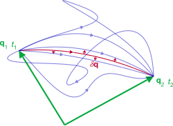
where the departure t1 and arrival t2 times are fixed.[1] The term "path" or "trajectory" refers to the time evolution of the system as a path through configuration space , in other words q(t) tracing out a path in . The path for which action is least is the path taken by the system.

From this principle, all equations of motion in classical mechanics can be derived. This approach can be extended to fields rather than a system of particles (see below), and underlies the path integral formulation of quantum mechanics,[11][12] and is used for calculating geodesic motion in general relativity.[13]
Hamiltonian-Jacobi mechanics edit
The invariance of the Hamiltonian (under addition of the partial time derivative of an arbitrary function of p, q, and t) allows the Hamiltonian in one set of coordinates q and momenta p to be transformed into a new set Q = Q(q, p, t) and P = P(q, p, t), in four possible ways:

With the restriction on P and Q such that the transformed Hamiltonian system is:

the above transformations are called canonical transformations, each function Gn is called a generating function of the "nth kind" or "type-n". The transformation of coordinates and momenta can allow simplification for solving Hamilton's equations for a given problem.
The choice of Q and P is completely arbitrary, but not every choice leads to a canonical transformation. One simple criterion for a transformation q → Q and p → P to be canonical is the Poisson bracket be unity,

for all i = 1, 2,...N. If this does not hold then the transformation is not canonical.[5]
By setting the canonically transformed Hamiltonian K = 0, and the type-2 generating function equal to Hamilton's principal function (also the action ) plus an arbitrary constant C:


the generalized momenta become:

and P is constant, then the Hamiltonian-Jacobi equation (HJE) can be derived from the type-2 canonical transformation:

where H is the Hamiltonian as before:

Another related function is Hamilton's characteristic function

used to solve the HJE by additive separation of variables for a time-independent Hamiltonian H.
The study of the solutions of the Hamilton–Jacobi equations leads naturally to the study of symplectic manifolds and symplectic topology.[14][15] In this formulation, the solutions of the Hamilton–Jacobi equations are the integral curves of Hamiltonian vector fields.
Routhian mechanics edit
Routhian mechanics is a hybrid formulation of Lagrangian and Hamiltonian mechanics, not often used but especially useful for removing cyclic coordinates.[citation needed] If the Lagrangian of a system has s cyclic coordinates q = q1, q2, ... qs with conjugate momenta p = p1, p2, ... ps, with the rest of the coordinates non-cyclic and denoted ζ = ζ1, ζ1, ..., ζN − s, they can be removed by introducing the Routhian:

which leads to a set of 2s Hamiltonian equations for the cyclic coordinates q,

and N − s Lagrangian equations in the non cyclic coordinates ζ.

Set up in this way, although the Routhian has the form of the Hamiltonian, it can be thought of a Lagrangian with N − s degrees of freedom.
The coordinates q do not have to be cyclic, the partition between which coordinates enter the Hamiltonian equations and those which enter the Lagrangian equations is arbitrary. It is simply convenient to let the Hamiltonian equations remove the cyclic coordinates, leaving the non cyclic coordinates to the Lagrangian equations of motion.
Appellian mechanics edit
Appell's equation of motion involve generalized accelerations, the second time derivatives of the generalized coordinates:

as well as generalized forces mentioned above in D'Alembert's principle. The equations are

where

is the acceleration of the k particle, the second time derivative of its position vector. Each acceleration ak is expressed in terms of the generalized accelerations αr, likewise each rk are expressed in terms the generalized coordinates qr.
Classical field theory edit
Lagrangian field theory edit
Generalized coordinates apply to discrete particles. For N scalar fields φi(r, t) where i = 1, 2, ... N, the Lagrangian density is a function of these fields and their space and time derivatives, and possibly the space and time coordinates themselves:


This scalar field formulation can be extended to vector fields, tensor fields, and spinor fields.
The Lagrangian is the volume integral of the Lagrangian density:[12][16]

Originally developed for classical fields, the above formulation is applicable to all physical fields in classical, quantum, and relativistic situations: such as Newtonian gravity, classical electromagnetism, general relativity, and quantum field theory. It is a question of determining the correct Lagrangian density to generate the correct field equation.
Hamiltonian field theory edit
The corresponding "momentum" field densities conjugate to the N scalar fields φi(r, t) are:[12]


The equations of motion are:


Again, the volume integral of the Hamiltonian density is the Hamiltonian

Symmetry, conservation, and Noether's theorem edit
- Symmetry transformations in classical space and time
Each transformation can be described by an operator (i.e. function acting on the position r or momentum p variables to change them). The following are the cases when the operator does not change r or p, i.e. symmetries.[11]
| Transformation | Operator | Position | Momentum |
|---|---|---|---|
| Translational symmetry | |||
| Time translation | |||
| Rotational invariance | |||
| Galilean transformations | |||
| Parity | |||
| T-symmetry |


where R(n̂, θ) is the rotation matrix about an axis defined by the unit vector n̂ and angle θ.
Noether's theorem states that a continuous symmetry transformation of the action corresponds to a conservation law, i.e. the action (and hence the Lagrangian) does not change under a transformation parameterized by a parameter s:
![{\displaystyle L[q(s,t),{\dot {q}}(s,t)]=L[q(t),{\dot {q}}(t)]}](https://wikimedia.org/api/rest_v1/media/math/render/svg/8a306c98f32aae1bd3da6bef5e96de807c6343bb)
See also edit
References and notes edit
- ^ a b Lanczos, Cornelius (1970). The variational principles of mechanics (4th ed.). New York: Dover Publications Inc. Introduction, pp. xxi–xxix. ISBN 0-486-65067-7.
- ^ Lanczos, Cornelius (1970). The variational principles of mechanics (4th ed.). New York: Dover Publications Inc. pp. 3–6. ISBN 978-0-486-65067-8.
- ^ Synge, J. L. (1960). "Classical dynamics". In Flügge, S. (ed.). Principles of Classical Mechanics and Field Theory / Prinzipien der Klassischen Mechanik und Feldtheorie. Encyclopedia of Physics / Handbuch der Physik. Vol. 2 / 3 / 1. Berlin, Heidelberg: Springer Berlin Heidelberg. doi:10.1007/978-3-642-45943-6. ISBN 978-3-540-02547-4. OCLC 165699220.
- ^ Kibble, Tom, and Berkshire, Frank H. "Classical Mechanics" (5th Edition). Singapore, World Scientific Publishing Company, 2004.
- ^ a b c d e Analytical Mechanics, L.N. Hand, J.D. Finch, Cambridge University Press, 2008, ISBN 978-0-521-57572-0
- ^ Torby, Bruce (1984). "Energy Methods". Advanced Dynamics for Engineers. HRW Series in Mechanical Engineering. United States of America: CBS College Publishing. ISBN 0-03-063366-4.
- ^ McGraw Hill Encyclopaedia of Physics (2nd Edition), C.B. Parker, 1994, ISBN 0-07-051400-3
- ^ Classical Mechanics, T.W.B. Kibble, European Physics Series, McGraw-Hill (UK), 1973, ISBN 0-07-084018-0
- ^ Penrose, R. (2007). The Road to Reality. Vintage books. p. 474. ISBN 978-0-679-77631-4.
- ^ Encyclopaedia of Physics (2nd Edition), R.G. Lerner, G.L. Trigg, VHC publishers, 1991, ISBN (Verlagsgesellschaft) 3-527-26954-1, ISBN (VHC Inc.) 0-89573-752-3
- ^ a b Quantum Mechanics, E. Abers, Pearson Ed., Addison Wesley, Prentice Hall Inc, 2004, ISBN 978-0-13-146100-0
- ^ a b c Quantum Field Theory, D. McMahon, Mc Graw Hill (US), 2008, ISBN 978-0-07-154382-8
- ^ Relativity, Gravitation, and Cosmology, R.J.A. Lambourne, Open University, Cambridge University Press, 2010, ISBN 978-0-521-13138-4
- ^ Arnolʹd, VI (1989). Mathematical methods of classical mechanics (2nd ed.). Springer. Chapter 8. ISBN 978-0-387-96890-2.
- ^ Doran, C; Lasenby, A (2003). Geometric algebra for physicists. Cambridge University Press. p. §12.3, pp. 432–439. ISBN 978-0-521-71595-9.
- ^ Gravitation, J.A. Wheeler, C. Misner, K.S. Thorne, W.H. Freeman & Co, 1973, ISBN 0-7167-0344-0