


Summary
Machine learning-based attention is a mechanism which intuitively mimics cognitive attention. It calculates "soft" weights for each word, more precisely for its embedding, in the context window. These weights can be computed either in parallel (such as in transformers) or sequentially (such as recurrent neural networks). "Soft" weights can change during each runtime, in contrast to "hard" weights, which are (pre-)trained and fine-tuned and remain frozen afterwards.
Attention was developed to address the weaknesses of leveraging information from the hidden outputs of recurrent neural networks. Recurrent neural networks favor more recent information contained in words at the end of a sentence, while information earlier in the sentence is expected to be attenuated. Attention allows the calculation of the hidden representation of a token equal access to any part of a sentence directly, rather than only through the previous hidden state.
Earlier uses attached this mechanism to a serial recurrent neural network's language translation system (below), but later uses in Transformers large language models removed the recurrent neural network and relied heavily on the faster parallel attention scheme.
Predecessors edit
Predecessors of the mechanism were used in recurrent neural networks which, however, calculated "soft" weights sequentially and, at each step, considered the current word and other words within the context window. They were known as multiplicative modules, sigma pi units,[1] and hyper-networks.[2] They have been used in long short-term memory (LSTM) networks, multi-sensory data processing (sound, images, video, and text) in perceivers, fast weight controller's memory,[3] reasoning tasks in differentiable neural computers, and neural Turing machines.[4][5][6][7][8]
Core calculations edit
The attention network was designed to identify the highest correlations amongst words within a sentence, assuming that it has learned those patterns from the training corpus. This correlation is captured in neuronal weights through backpropagation, either from self-supervised pretraining or supervised fine-tuning.
The example below (a encoder-only QKV variant of an attention network) shows how correlations are identified once a network has been trained and has the right weights. When looking at the word "that" in the sentence "see that girl run", the network should be able to identify "girl" as a highly correlated word. For simplicity this example focuses on the word "that", but in reality all words receive this treatment in parallel and the resulting soft-weights and context vectors are stacked into matrices for further task-specific use.

The sentence is sent through 3 parallel streams (left), which emerge at the end as the context vector (right). The word embedding size is 300 and the neuron count is 100 in each sub-network of the attention head.
- The capital letter X denotes a matrix sized 4 × 300, consisting of the embeddings of all four words.
- The small underlined letter x denotes the embedding vector (sized 300) of the word "that".
- The attention head includes three (vertically arranged in the illustration) sub-networks, each having 100 neurons, being Wq, Wk and Wv their respective weight matrices, all them sized 300 × 100.
- q (from "query") is a vector sized 100, Wk ("key") and Wv ("value") are 4x100 matrices.
- The asterisk within parenthesis "(*)" denotes the softmax( qWk / √100 ). Softmax result is a vector sized 4 that later on is multiplied by the matrix V=XWv to obtain the context vector.
- Rescaling by √100 prevents a high variance in qWkT that would allow a single word to excessively dominate the softmax resulting in attention to only one word, as a discrete hard max would do.
Notation: the commonly written row-wise softmax formula above assumes that vectors are rows, which contradicts the standard math notation of column vectors. More correctly, we should take the transpose of the context vector and use the column-wise softmax, resulting in the more correct form
The query vector is compared (via dot product) with each word in the keys. This helps the model discover the most relevant word for the query word. In this case "girl" was determined to be the most relevant word for "that". The result (size 4 in this case) is run through the softmax function, producing a vector of size 4 with probabilities summing to 1. Multiplying this against the value matrix effectively amplifies the signal for the most important words in the sentence and diminishes the signal for less important words.[5]
The structure of the input data is captured in the Wq and Wk weights, and the Wv weights express that structure in terms of more meaningful features for the task being trained for. For this reason, the attention head components are called Query (Wq), Key (Wk), and Value (Wv)—a loose and possibly misleading analogy with relational database systems.
Note that the context vector for "that" does not rely on context vectors for the other words; therefore the context vectors of all words can be calculated using the whole matrix X, which includes all the word embeddings, instead of a single word's embedding vector x in the formula above, thus parallelizing the calculations. Now, the softmax can be interpreted as a matrix softmax acting on separate rows. This is a huge advantage over recurrent networks which must operate sequentially.
The common query-key analogy with database queries suggests an asymmetric role for these vectors, where one item of interest (the query) is matched against all possible items (the keys). However, parallel calculations matches all words of the sentence with itself; therefore the roles of these vectors are symmetric. Possibly because the simplistic database analogy is flawed, much effort has gone into understand Attention further by studying their roles in focused settings, such as in-context learning,[9] masked language tasks,[10] stripped down transformers,[11] bigram statistics,[12] pairwise convolutions,[13] and arithmetic factoring.[14]
A language translation example edit
To build a machine that translates English to French, an attention unit is grafted to the basic Encoder-Decoder (diagram below). In the simplest case, the attention unit consists of dot products of the recurrent encoder states and does not need training. In practice, the attention unit consists of 3 trained, fully-connected neural network layers called query, key, and value.
![Encoder-decoder with attention.[15] The left part (black lines) is the encoder-decoder, the middle part (orange lines) is the attention unit, and the right part (in grey & colors) is the computed data. Grey regions in H matrix and w vector are zero values. Numerical subscripts indicate vector sizes while lettered subscripts i and i − 1 indicate time steps.](http://upload.wikimedia.org/wikipedia/commons/f/f7/Attention-1-sn.png)
| Label | Description |
|---|---|
| 100 | Max. sentence length |
| 300 | Embedding size (word dimension) |
| 500 | Length of hidden vector |
| 9k, 10k | Dictionary size of input & output languages respectively. |
| x, Y | 9k and 10k 1-hot dictionary vectors. x → x implemented as a lookup table rather than vector multiplication. Y is the 1-hot maximizer of the linear Decoder layer D; that is, it takes the argmax of D's linear layer output. |
| x | 300-long word embedding vector. The vectors are usually pre-calculated from other projects such as GloVe or Word2Vec. |
| h | 500-long encoder hidden vector. At each point in time, this vector summarizes all the preceding words before it. The final h can be viewed as a "sentence" vector, or a thought vector as Hinton calls it. |
| s | 500-long decoder hidden state vector. |
| E | 500 neuron recurrent neural network encoder. 500 outputs. Input count is 800–300 from source embedding + 500 from recurrent connections. The encoder feeds directly into the decoder only to initialize it, but not thereafter; hence, that direct connection is shown very faintly. |
| D | 2-layer decoder. The recurrent layer has 500 neurons and the fully-connected linear layer has 10k neurons (the size of the target vocabulary).[16] The linear layer alone has 5 million (500 × 10k) weights – ~10 times more weights than the recurrent layer. |
| score | 100-long alignment score |
| w | 100-long vector attention weight. These are "soft" weights which changes during the forward pass, in contrast to "hard" neuronal weights that change during the learning phase. |
| A | Attention module – this can be a dot product of recurrent states, or the query-key-value fully-connected layers. The output is a 100-long vector w. |
| H | 500×100. 100 hidden vectors h concatenated into a matrix |
| c | 500-long context vector = H * w. c is a linear combination of h vectors weighted by w. |
Viewed as a matrix, the attention weights show how the network adjusts its focus according to context.[17]
| I | love | you | |
| je | 0.94 | 0.02 | 0.04 |
| t' | 0.11 | 0.01 | 0.88 |
| aime | 0.03 | 0.95 | 0.02 |
This view of the attention weights addresses the neural network "explainability" problem. Networks that perform verbatim translation without regard to word order would show the highest scores along the (dominant) diagonal of the matrix. The off-diagonal dominance shows that the attention mechanism is more nuanced. On the first pass through the decoder, 94% of the attention weight is on the first English word "I", so the network offers the word "je". On the second pass of the decoder, 88% of the attention weight is on the third English word "you", so it offers "t'". On the last pass, 95% of the attention weight is on the second English word "love", so it offers "aime".
Variants edit
Many variants of attention implement soft weights, such as
- "internal spotlights of attention"[18] generated by fast weight programmers or fast weight controllers (1992)[3] (also known as transformers with "linearized self-attention"[19][20]). A slow neural network learns by gradient descent to program the fast weights of another neural network through outer products of self-generated activation patterns called "FROM" and "TO" which in transformer terminology are called "key" and "value." This fast weight "attention mapping" is applied to queries.
- Bahdanau-style attention,[17] also referred to as additive attention,
- Luong-style attention,[21] which is known as multiplicative attention,
- highly parallelizable self-attention introduced in 2016 as decomposable attention[22] and successfully used in transformers a year later.
For convolutional neural networks, attention mechanisms can be distinguished by the dimension on which they operate, namely: spatial attention,[23] channel attention,[24] or combinations.[25][26]
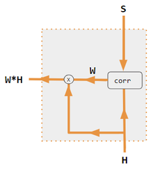
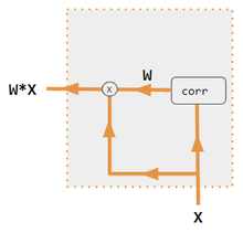
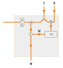
These variants recombine the encoder-side inputs to redistribute those effects to each target output. Often, a correlation-style matrix of dot products provides the re-weighting coefficients. In the figures below, W is the matrix of context attention weights, similar to the formula in Core Calculations section above.
| 1. encoder-decoder dot product | 2. encoder-decoder QKV | 3. encoder-only dot product | 4. encoder-only QKV | 5. Pytorch tutorial |
|---|---|---|---|---|
 |
 |
 |
 |
 |
| Label | Description |
|---|---|
| Variables X, H, S, T | Upper case variables represent the entire sentence, and not just the current word. For example, H is a matrix of the encoder hidden state—one word per column. |
| S, T | S, decoder hidden state; T, target word embedding. In the Pytorch Tutorial variant training phase, T alternates between 2 sources depending on the level of teacher forcing used. T could be the embedding of the network's output word; i.e. embedding(argmax(FC output)). Alternatively with teacher forcing, T could be the embedding of the known correct word which can occur with a constant forcing probability, say 1/2. |
| X, H | H, encoder hidden state; X, input word embeddings. |
| W | Attention coefficients |
| Qw, Kw, Vw, FC | Weight matrices for query, key, value respectively. FC is a fully-connected weight matrix. |
| ⊕, ⊗ | ⊕, vector concatenation; ⊗, matrix multiplication. |
| corr | Column-wise softmax(matrix of all combinations of dot products). The dot products are xi * xj in variant #3, hi* sj in variant 1, and column i ( Kw * H ) * column j ( Qw * S ) in variant 2, and column i ( Kw * X ) * column j ( Qw * X ) in variant 4. Variant 5 uses a fully-connected layer to determine the coefficients. If the variant is QKV, then the dot products are normalized by the √d where d is the height of the QKV matrices. |
Mathematical representation edit
Standard Scaled Dot-Product Attention edit


Multi-Head Attention edit


Bahdanau (Additive) Attention edit


Luong Attention (General) edit


See also edit
References edit
- ^ Rumelhart, David E.; Mcclelland, James L.; Group, PDP Research (1987-07-29). Parallel Distributed Processing, Volume 1: Explorations in the Microstructure of Cognition: Foundations, Chapter 2 (PDF). Cambridge, Mass: Bradford Books. ISBN 978-0-262-68053-0.
- ^ Yann Lecun (2020). Deep Learning course at NYU, Spring 2020, video lecture Week 6. Event occurs at 53:00. Retrieved 2022-03-08.
- ^ a b Schmidhuber, Jürgen (1992). "Learning to control fast-weight memories: an alternative to recurrent nets". Neural Computation. 4 (1): 131–139. doi:10.1162/neco.1992.4.1.131. S2CID 16683347.
- ^ Graves, Alex; Wayne, Greg; Reynolds, Malcolm; Harley, Tim; Danihelka, Ivo; Grabska-Barwińska, Agnieszka; Colmenarejo, Sergio Gómez; Grefenstette, Edward; Ramalho, Tiago; Agapiou, John; Badia, Adrià Puigdomènech; Hermann, Karl Moritz; Zwols, Yori; Ostrovski, Georg; Cain, Adam; King, Helen; Summerfield, Christopher; Blunsom, Phil; Kavukcuoglu, Koray; Hassabis, Demis (2016-10-12). "Hybrid computing using a neural network with dynamic external memory". Nature. 538 (7626): 471–476. Bibcode:2016Natur.538..471G. doi:10.1038/nature20101. ISSN 1476-4687. PMID 27732574. S2CID 205251479.
- ^ a b Vaswani, Ashish; Shazeer, Noam; Parmar, Niki; Uszkoreit, Jakob; Jones, Llion; Gomez, Aidan N; Kaiser, Łukasz; Polosukhin, Illia (2017). "Attention is All you Need" (PDF). Advances in Neural Information Processing Systems. 30. Curran Associates, Inc.
- ^ Ramachandran, Prajit; Parmar, Niki; Vaswani, Ashish; Bello, Irwan; Levskaya, Anselm; Shlens, Jonathon (2019-06-13). "Stand-Alone Self-Attention in Vision Models". arXiv:1906.05909 [cs.CV].
- ^ Jaegle, Andrew; Gimeno, Felix; Brock, Andrew; Zisserman, Andrew; Vinyals, Oriol; Carreira, Joao (2021-06-22). "Perceiver: General Perception with Iterative Attention". arXiv:2103.03206 [cs.CV].
- ^ Ray, Tiernan. "Google's Supermodel: DeepMind Perceiver is a step on the road to an AI machine that could process anything and everything". ZDNet. Retrieved 2021-08-19.
- ^ Zhang, Ruiqi (2024). "Trained Transformers Learn Linear Models In-Context" (PDF). Journal of Machine Learning Research 1-55. 25.
- ^ Rende, Riccardo (2023). "Mapping of attention mechanisms to a generalized Potts model". arXiv:2304.07235.
- ^ He, Bobby (2023). "Simplifying Transformers Blocks". arXiv:2311.01906.
- ^ "Transformer Circuits". transformer-circuits.pub.
- ^ Transformer Neural Network Derived From Scratch. 2023. Event occurs at 05:30. Retrieved 2024-04-07.
- ^ Charton, François (2023). "Learning the Greatest Common Divisor: Explaining Transformer Predictions". arXiv:2308.15594.
- ^ Britz, Denny; Goldie, Anna; Luong, Minh-Thanh; Le, Quoc (2017-03-21). "Massive Exploration of Neural Machine Translation Architectures". arXiv:1703.03906 [cs.CV].
- ^ "Pytorch.org seq2seq tutorial". Retrieved December 2, 2021.
- ^ a b c Bahdanau, Dzmitry; Cho, Kyunghyun; Bengio, Yoshua (2014). "Neural Machine Translation by Jointly Learning to Align and Translate". arXiv:1409.0473 [cs.CL].
- ^ Schmidhuber, Jürgen (1993). "Reducing the ratio between learning complexity and number of time-varying variables in fully recurrent nets". ICANN 1993. Springer. pp. 460–463.
- ^ Schlag, Imanol; Irie, Kazuki; Schmidhuber, Jürgen (2021). "Linear Transformers Are Secretly Fast Weight Programmers". ICML 2021. Springer. pp. 9355–9366.
- ^ Choromanski, Krzysztof; Likhosherstov, Valerii; Dohan, David; Song, Xingyou; Gane, Andreea; Sarlos, Tamas; Hawkins, Peter; Davis, Jared; Mohiuddin, Afroz; Kaiser, Lukasz; Belanger, David; Colwell, Lucy; Weller, Adrian (2020). "Rethinking Attention with Performers". arXiv:2009.14794 [cs.CL].
- ^ a b c Luong, Minh-Thang (2015-09-20). "Effective Approaches to Attention-Based Neural Machine Translation". arXiv:1508.04025v5 [cs.CL].
- ^ "Papers with Code - A Decomposable Attention Model for Natural Language Inference". paperswithcode.com.
- ^ Zhu, Xizhou; Cheng, Dazhi; Zhang, Zheng; Lin, Stephen; Dai, Jifeng (2019). "An Empirical Study of Spatial Attention Mechanisms in Deep Networks". 2019 IEEE/CVF International Conference on Computer Vision (ICCV). pp. 6687–6696. arXiv:1904.05873. doi:10.1109/ICCV.2019.00679. ISBN 978-1-7281-4803-8. S2CID 118673006.
- ^ Hu, Jie; Shen, Li; Sun, Gang (2018). "Squeeze-and-Excitation Networks". 2018 IEEE/CVF Conference on Computer Vision and Pattern Recognition. pp. 7132–7141. arXiv:1709.01507. doi:10.1109/CVPR.2018.00745. ISBN 978-1-5386-6420-9. S2CID 206597034.
- ^ Woo, Sanghyun; Park, Jongchan; Lee, Joon-Young; Kweon, In So (2018-07-18). "CBAM: Convolutional Block Attention Module". arXiv:1807.06521 [cs.CV].
- ^ Georgescu, Mariana-Iuliana; Ionescu, Radu Tudor; Miron, Andreea-Iuliana; Savencu, Olivian; Ristea, Nicolae-Catalin; Verga, Nicolae; Khan, Fahad Shahbaz (2022-10-12). "Multimodal Multi-Head Convolutional Attention with Various Kernel Sizes for Medical Image Super-Resolution". arXiv:2204.04218 [eess.IV].
- ^ Neil Rhodes (2021). CS 152 NN—27: Attention: Keys, Queries, & Values. Event occurs at 06:30. Retrieved 2021-12-22.
- ^ Alfredo Canziani & Yann Lecun (2021). NYU Deep Learning course, Spring 2020. Event occurs at 05:30. Retrieved 2021-12-22.
- ^ Alfredo Canziani & Yann Lecun (2021). NYU Deep Learning course, Spring 2020. Event occurs at 20:15. Retrieved 2021-12-22.
- ^ Robertson, Sean. "NLP From Scratch: Translation With a Sequence To Sequence Network and Attention". pytorch.org. Retrieved 2021-12-22.
External links edit
- Dan Jurafsky and James H. Martin (2022) Speech and Language Processing (3rd ed. draft, January 2022), ch. 10.4 Attention and ch. 9.7 Self-Attention Networks: Transformers
- Alex Graves (4 May 2020), Attention and Memory in Deep Learning (video lecture), DeepMind / UCL, via YouTube