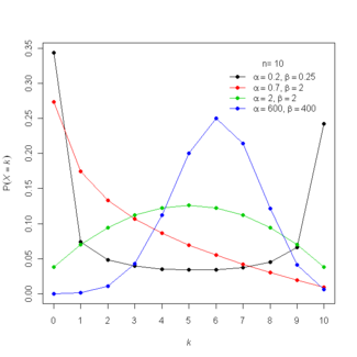
In probability theory and statistics , the beta-binomial distribution is a family of discrete probability distributions on a finite support of non-negative integers arising when the probability of success in each of a fixed or known number of Bernoulli trials is either unknown or random. The beta-binomial distribution is the binomial distribution in which the probability of success at each of n trials is not fixed but randomly drawn from a beta distribution . It is frequently used in Bayesian statistics , empirical Bayes methods and classical statistics to capture overdispersion in binomial type distributed data.
Probability mass function
Cumulative distribution function
Notation
B
e
t
a
B
i
n
(
n
,
α
,
β
)
{\displaystyle \mathrm {BetaBin} (n,\alpha ,\beta )}
Parameters
n ∈ N 0
α
>
0
{\displaystyle \alpha >0}
real )
β
>
0
{\displaystyle \beta >0}
real ) Support
x ∈ { 0, …, n } PMF
(
n
x
)
B
(
x
+
α
,
n
−
x
+
β
)
B
(
α
,
β
)
{\displaystyle {\binom {n}{x}}{\frac {\mathrm {B} (x+\alpha ,n-x+\beta )}{\mathrm {B} (\alpha ,\beta )}}\!}
B
(
x
,
y
)
=
Γ
(
x
)
Γ
(
y
)
Γ
(
x
+
y
)
{\displaystyle \mathrm {B} (x,y)={\frac {\Gamma (x)\,\Gamma (y)}{\Gamma (x+y)}}}
beta function CDF
{
0
,
x
<
0
(
n
x
)
B
(
x
+
α
,
n
−
x
+
β
)
B
(
α
,
β
)
3
F
2
(
a
;
b
;
x
)
,
0
≤
x
<
n
1
,
x
≥
n
{\displaystyle {\begin{cases}0,&x<0\\{\binom {n}{x}}{\tfrac {\mathrm {B} (x+\alpha ,n-x+\beta )}{\mathrm {B} (\alpha ,\beta )}}{}_{3}\!F_{2}({\boldsymbol {a}};{\boldsymbol {b}};x),&0\leq x<n\\1,&x\geq n\end{cases}}}
3 F 2 (a ;b ;x) is the generalized hypergeometric function
3
F
2
(
1
,
−
x
,
n
−
x
+
β
;
n
−
x
+
1
,
1
−
x
−
α
;
1
)
{\displaystyle {}_{3}\!F_{2}(1,-x,n\!-\!x\!+\!\beta ;n\!-\!x\!+\!1,1\!-\!x\!-\!\alpha ;1)\!}
Mean
n
α
α
+
β
{\displaystyle {\frac {n\alpha }{\alpha +\beta }}\!}
Variance
n
α
β
(
α
+
β
+
n
)
(
α
+
β
)
2
(
α
+
β
+
1
)
{\displaystyle {\frac {n\alpha \beta (\alpha +\beta +n)}{(\alpha +\beta )^{2}(\alpha +\beta +1)}}\!}
Skewness
(
α
+
β
+
2
n
)
(
β
−
α
)
(
α
+
β
+
2
)
1
+
α
+
β
n
α
β
(
n
+
α
+
β
)
{\displaystyle {\tfrac {(\alpha +\beta +2n)(\beta -\alpha )}{(\alpha +\beta +2)}}{\sqrt {\tfrac {1+\alpha +\beta }{n\alpha \beta (n+\alpha +\beta )}}}\!}
Excess kurtosis
See text MGF
2
F
1
(
−
n
,
α
;
α
+
β
;
1
−
e
t
)
{\displaystyle _{2}F_{1}(-n,\alpha ;\alpha +\beta ;1-e^{t})\!}
2
F
1
{\displaystyle _{2}F_{1}}
hypergeometric function CF
2
F
1
(
−
n
,
α
;
α
+
β
;
1
−
e
i
t
)
{\displaystyle _{2}F_{1}(-n,\alpha ;\alpha +\beta ;1-e^{it})\!}
PGF
2
F
1
(
−
n
,
α
;
α
+
β
;
1
−
z
)
{\displaystyle _{2}F_{1}(-n,\alpha ;\alpha +\beta ;1-z)\!}
The beta-binomial is a one-dimensional version of the Dirichlet-multinomial distribution as the binomial and beta distributions are univariate versions of the multinomial and Dirichlet distributions respectively. The special case where α and β are integers is also known as the negative hypergeometric distribution .
Motivation and derivation
edit
As a compound distribution
edit
The Beta distribution is a conjugate distribution of the binomial distribution . This fact leads to an analytically tractable compound distribution where one can think of the
p
{\displaystyle p}
x
{\displaystyle x}
n
{\displaystyle n}
f
(
x
∣
n
,
α
,
β
)
=
∫
0
1
B
i
n
(
x
|
n
,
p
)
B
e
t
a
(
p
∣
α
,
β
)
d
p
=
(
n
x
)
1
B
(
α
,
β
)
∫
0
1
p
x
+
α
−
1
(
1
−
p
)
n
−
x
+
β
−
1
d
p
=
(
n
x
)
B
(
x
+
α
,
n
−
x
+
β
)
B
(
α
,
β
)
.
{\displaystyle {\begin{aligned}f(x\mid n,\alpha ,\beta )&=\int _{0}^{1}\mathrm {Bin} (x|n,p)\mathrm {Beta} (p\mid \alpha ,\beta )\,dp\\[6pt]&={n \choose x}{\frac {1}{\mathrm {B} (\alpha ,\beta )}}\int _{0}^{1}p^{x+\alpha -1}(1-p)^{n-x+\beta -1}\,dp\\[6pt]&={n \choose x}{\frac {\mathrm {B} (x+\alpha ,n-x+\beta )}{\mathrm {B} (\alpha ,\beta )}}.\end{aligned}}}
Using the properties of the beta function , this can alternatively be written
f
(
x
∣
n
,
α
,
β
)
=
Γ
(
n
+
1
)
Γ
(
x
+
1
)
Γ
(
n
−
x
+
1
)
Γ
(
x
+
α
)
Γ
(
n
−
x
+
β
)
Γ
(
n
+
α
+
β
)
Γ
(
α
+
β
)
Γ
(
α
)
Γ
(
β
)
{\displaystyle f(x\mid n,\alpha ,\beta )={\frac {\Gamma (n+1)}{\Gamma (x+1)\Gamma (n-x+1)}}{\frac {\Gamma (x+\alpha )\Gamma (n-x+\beta )}{\Gamma (n+\alpha +\beta )}}{\frac {\Gamma (\alpha +\beta )}{\Gamma (\alpha )\Gamma (\beta )}}}
As an urn model
edit
The beta-binomial distribution can also be motivated via an urn model for positive integer values of α and β , known as the Pólya urn model . Specifically, imagine an urn containing α red balls and β black balls, where random draws are made. If a red ball is observed, then two red balls are returned to the urn. Likewise, if a black ball is drawn, then two black balls are returned to the urn. If this is repeated n times, then the probability of observing x red balls follows a beta-binomial distribution with parameters n , α and β .
By contrast, if the random draws are with simple replacement (no balls over and above the observed ball are added to the urn), then the distribution follows a binomial distribution and if the random draws are made without replacement, the distribution follows a hypergeometric distribution .
Moments and properties
edit
The first three raw moments are
μ
1
=
n
α
α
+
β
μ
2
=
n
α
[
n
(
1
+
α
)
+
β
]
(
α
+
β
)
(
1
+
α
+
β
)
μ
3
=
n
α
[
n
2
(
1
+
α
)
(
2
+
α
)
+
3
n
(
1
+
α
)
β
+
β
(
β
−
α
)
]
(
α
+
β
)
(
1
+
α
+
β
)
(
2
+
α
+
β
)
{\displaystyle {\begin{aligned}\mu _{1}&={\frac {n\alpha }{\alpha +\beta }}\\[8pt]\mu _{2}&={\frac {n\alpha [n(1+\alpha )+\beta ]}{(\alpha +\beta )(1+\alpha +\beta )}}\\[8pt]\mu _{3}&={\frac {n\alpha [n^{2}(1+\alpha )(2+\alpha )+3n(1+\alpha )\beta +\beta (\beta -\alpha )]}{(\alpha +\beta )(1+\alpha +\beta )(2+\alpha +\beta )}}\end{aligned}}}
and the kurtosis is
β
2
=
(
α
+
β
)
2
(
1
+
α
+
β
)
n
α
β
(
α
+
β
+
2
)
(
α
+
β
+
3
)
(
α
+
β
+
n
)
[
(
α
+
β
)
(
α
+
β
−
1
+
6
n
)
+
3
α
β
(
n
−
2
)
+
6
n
2
−
3
α
β
n
(
6
−
n
)
α
+
β
−
18
α
β
n
2
(
α
+
β
)
2
]
.
{\displaystyle \beta _{2}={\frac {(\alpha +\beta )^{2}(1+\alpha +\beta )}{n\alpha \beta (\alpha +\beta +2)(\alpha +\beta +3)(\alpha +\beta +n)}}\left[(\alpha +\beta )(\alpha +\beta -1+6n)+3\alpha \beta (n-2)+6n^{2}-{\frac {3\alpha \beta n(6-n)}{\alpha +\beta }}-{\frac {18\alpha \beta n^{2}}{(\alpha +\beta )^{2}}}\right].}
Letting
p
=
α
α
+
β
{\displaystyle p={\frac {\alpha }{\alpha +\beta }}\!}
μ
=
n
α
α
+
β
=
n
p
{\displaystyle \mu ={\frac {n\alpha }{\alpha +\beta }}=np\!}
and the variance as
σ
2
=
n
α
β
(
α
+
β
+
n
)
(
α
+
β
)
2
(
α
+
β
+
1
)
=
n
p
(
1
−
p
)
α
+
β
+
n
α
+
β
+
1
=
n
p
(
1
−
p
)
[
1
+
(
n
−
1
)
ρ
]
{\displaystyle \sigma ^{2}={\frac {n\alpha \beta (\alpha +\beta +n)}{(\alpha +\beta )^{2}(\alpha +\beta +1)}}=np(1-p){\frac {\alpha +\beta +n}{\alpha +\beta +1}}=np(1-p)[1+(n-1)\rho ]\!}
where
ρ
=
1
α
+
β
+
1
{\displaystyle \rho ={\tfrac {1}{\alpha +\beta +1}}\!}
ρ
{\displaystyle \rho \;\!}
n
=
1
{\displaystyle n=1}
Factorial moments
edit
The r factorial moment of a Beta-binomial random variable X
E
[
(
X
)
r
]
=
n
!
(
n
−
r
)
!
B
(
α
+
r
,
β
)
B
(
α
,
β
)
=
(
n
)
r
B
(
α
+
r
,
β
)
B
(
α
,
β
)
{\displaystyle \operatorname {E} {\bigl [}(X)_{r}{\bigr ]}={\frac {n!}{(n-r)!}}{\frac {B(\alpha +r,\beta )}{B(\alpha ,\beta )}}=(n)_{r}{\frac {B(\alpha +r,\beta )}{B(\alpha ,\beta )}}}
Point estimates
edit
Method of moments
edit
The method of moments estimates can be gained by noting the first and second moments of the beta-binomial and setting those equal to the sample moments
m
1
{\displaystyle m_{1}}
m
2
{\displaystyle m_{2}}
α
^
=
n
m
1
−
m
2
n
(
m
2
m
1
−
m
1
−
1
)
+
m
1
β
^
=
(
n
−
m
1
)
(
n
−
m
2
m
1
)
n
(
m
2
m
1
−
m
1
−
1
)
+
m
1
.
{\displaystyle {\begin{aligned}{\widehat {\alpha }}&={\frac {nm_{1}-m_{2}}{n({\frac {m_{2}}{m_{1}}}-m_{1}-1)+m_{1}}}\\[5pt]{\widehat {\beta }}&={\frac {(n-m_{1})(n-{\frac {m_{2}}{m_{1}}})}{n({\frac {m_{2}}{m_{1}}}-m_{1}-1)+m_{1}}}.\end{aligned}}}
These estimates can be non-sensically negative which is evidence that the data is either undispersed or underdispersed relative to the binomial distribution. In this case, the binomial distribution and the hypergeometric distribution are alternative candidates respectively.
Maximum likelihood estimation
edit
While closed-form maximum likelihood estimates are impractical, given that the pdf consists of common functions (gamma function and/or Beta functions), they can be easily found via direct numerical optimization. Maximum likelihood estimates from empirical data can be computed using general methods for fitting multinomial Pólya distributions, methods for which are described in (Minka 2003).
The R package VGAM through the function vglm, via maximum likelihood, facilitates the fitting of glm type models with responses distributed according to the beta-binomial distribution. There is no requirement that n is fixed throughout the observations.
Example: Sex ratio heterogeneity
edit
The following data gives the number of male children among the first 12 children of family size 13 in 6115 families taken from hospital records in 19th century Saxony (Sokal and Rohlf, p. 59 from Lindsey). The 13th child is ignored to blunt the effect of families non-randomly stopping when a desired gender is reached.
Males 0
1
2
3
4
5
6
7
8
9
10
11
12
Families 3
24
104
286
670
1033
1343
1112
829
478
181
45
7
The first two sample moments are
m
1
=
6.23
m
2
=
42.31
n
=
12
{\displaystyle {\begin{aligned}m_{1}&=6.23\\m_{2}&=42.31\\n&=12\end{aligned}}}
and therefore the method of moments estimates are
α
^
=
34.1350
β
^
=
31.6085.
{\displaystyle {\begin{aligned}{\widehat {\alpha }}&=34.1350\\{\widehat {\beta }}&=31.6085.\end{aligned}}}
The maximum likelihood estimates can be found numerically
α
^
m
l
e
=
34.09558
β
^
m
l
e
=
31.5715
{\displaystyle {\begin{aligned}{\widehat {\alpha }}_{\mathrm {mle} }&=34.09558\\{\widehat {\beta }}_{\mathrm {mle} }&=31.5715\end{aligned}}}
and the maximized log-likelihood is
log
L
=
−
12492.9
{\displaystyle \log {\mathcal {L}}=-12492.9}
from which we find the AIC
A
I
C
=
24989.74.
{\displaystyle {\mathit {AIC}}=24989.74.}
The AIC for the competing binomial model is AIC = 25070.34 and thus we see that the beta-binomial model provides a superior fit to the data i.e. there is evidence for overdispersion. Trivers and Willard postulate a theoretical justification for heterogeneity in gender-proneness among mammalian offspring.
The superior fit is evident especially among the tails
Males 0
1
2
3
4
5
6
7
8
9
10
11
12
Observed Families 3
24
104
286
670
1033
1343
1112
829
478
181
45
7
Fitted Expected (Beta-Binomial) 2.3
22.6
104.8
310.9
655.7
1036.2
1257.9
1182.1
853.6
461.9
177.9
43.8
5.2
Fitted Expected (Binomial p = 0.519215) 0.9
12.1
71.8
258.5
628.1
1085.2
1367.3
1265.6
854.2
410.0
132.8
26.1
2.3
Role in Bayesian statistics
edit
The beta-binomial distribution plays a prominent role in the Bayesian estimation of a Bernoulli success probability
p
{\displaystyle p}
X
=
{
X
1
,
X
2
,
⋯
X
n
1
}
{\displaystyle \mathbf {X} =\{X_{1},X_{2},\cdots X_{n_{1}}\}}
sample of independent and identically distributed Bernoulli random variables
X
i
∼
Bernoulli
(
p
)
{\displaystyle X_{i}\sim {\text{Bernoulli}}(p)}
p
{\displaystyle p}
prior distribution
p
∼
Beta
(
α
,
β
)
{\displaystyle p\sim {\text{Beta}}(\alpha ,\beta )}
Y
1
=
∑
i
=
1
n
1
X
i
{\displaystyle Y_{1}=\sum _{i=1}^{n_{1}}X_{i}}
compounding , the prior predictive distribution of
Y
1
∼
BetaBin
(
n
1
,
α
,
β
)
{\displaystyle Y_{1}\sim {\text{BetaBin}}(n_{1},\alpha ,\beta )}
After observing
Y
1
{\displaystyle Y_{1}}
posterior distribution for
p
{\displaystyle p}
f
(
p
|
X
,
α
,
β
)
∝
(
∏
i
=
1
n
1
p
x
i
(
1
−
p
)
1
−
x
i
)
p
α
−
1
(
1
−
p
)
β
−
1
=
C
p
∑
x
i
+
α
−
1
(
1
−
p
)
n
1
−
∑
x
i
+
β
−
1
=
C
p
y
1
+
α
−
1
(
1
−
p
)
n
1
−
y
1
+
β
−
1
{\displaystyle {\begin{aligned}f(p|\mathbf {X} ,\alpha ,\beta )&\propto \left(\prod _{i=1}^{n_{1}}p^{x_{i}}(1-p)^{1-x_{i}}\right)p^{\alpha -1}(1-p)^{\beta -1}\\&=Cp^{\sum x_{i}+\alpha -1}(1-p)^{n_{1}-\sum x_{i}+\beta -1}\\&=Cp^{y_{1}+\alpha -1}(1-p)^{n_{1}-y_{1}+\beta -1}\end{aligned}}}
where
C
{\displaystyle C}
B
e
t
a
(
y
1
+
α
,
n
1
−
y
1
+
β
)
{\displaystyle \mathrm {Beta} (y_{1}+\alpha ,n_{1}-y_{1}+\beta )}
Thus, again through compounding, we find that the posterior predictive distribution of a sum of a future sample of size
n
2
{\displaystyle n_{2}}
B
e
r
n
o
u
l
l
i
(
p
)
{\displaystyle \mathrm {Bernoulli} (p)}
Y
2
∼
B
e
t
a
B
i
n
(
n
2
,
y
1
+
α
,
n
1
−
y
1
+
β
)
{\displaystyle Y_{2}\sim \mathrm {BetaBin} (n_{2},y_{1}+\alpha ,n_{1}-y_{1}+\beta )}
Generating random variates
edit
Related distributions
edit
B
e
t
a
B
i
n
(
1
,
α
,
β
)
∼
B
e
r
n
o
u
l
l
i
(
p
)
{\displaystyle \mathrm {BetaBin} (1,\alpha ,\beta )\sim \mathrm {Bernoulli} (p)\,}
p
=
α
α
+
β
{\displaystyle p={\frac {\alpha }{\alpha +\beta }}\,}
B
e
t
a
B
i
n
(
n
,
1
,
1
)
∼
U
(
0
,
n
)
{\displaystyle \mathrm {BetaBin} (n,1,1)\sim U(0,n)\,}
U
(
a
,
b
)
{\displaystyle U(a,b)\,}
discrete uniform distribution .
lim
s
→
∞
B
e
t
a
B
i
n
(
n
,
p
s
,
(
1
−
p
)
s
)
∼
B
(
n
,
p
)
{\displaystyle \lim _{s\rightarrow \infty }\mathrm {BetaBin} (n,ps,(1-p)s)\sim \mathrm {B} (n,p)\,}
p
=
α
α
+
β
{\displaystyle p={\frac {\alpha }{\alpha +\beta }}\,}
s
=
α
+
β
{\displaystyle s=\alpha +\beta \,}
B
(
n
,
p
)
{\displaystyle \mathrm {B} (n,p)\,}
binomial distribution .
lim
n
→
∞
B
e
t
a
B
i
n
(
n
,
α
,
n
p
(
1
−
p
)
)
∼
N
B
(
α
,
p
)
{\displaystyle \lim _{n\rightarrow \infty }\mathrm {BetaBin} (n,\alpha ,{\frac {np}{(1-p)}})\sim \mathrm {NB} (\alpha ,p)\,}
N
B
(
α
,
p
)
{\displaystyle \mathrm {NB} (\alpha ,p)\,}
negative binomial distribution . See also
edit
References
edit
External links
edit
Using the Beta-binomial distribution to assess performance of a biometric identification device
Fastfit contains Matlab code for fitting Beta-Binomial distributions (in the form of two-dimensional Pólya distributions) to data.
Interactive graphic: Univariate Distribution Relationships
Beta-binomial functions in VGAM R package
Beta-binomial distribution in Sandia National Labs Cognitive Foundry Java library


![{\displaystyle {\begin{aligned}f(x\mid n,\alpha ,\beta )&=\int _{0}^{1}\mathrm {Bin} (x|n,p)\mathrm {Beta} (p\mid \alpha ,\beta )\,dp\\[6pt]&={n \choose x}{\frac {1}{\mathrm {B} (\alpha ,\beta )}}\int _{0}^{1}p^{x+\alpha -1}(1-p)^{n-x+\beta -1}\,dp\\[6pt]&={n \choose x}{\frac {\mathrm {B} (x+\alpha ,n-x+\beta )}{\mathrm {B} (\alpha ,\beta )}}.\end{aligned}}}](https://wikimedia.org/api/rest_v1/media/math/render/svg/26b9fd585e7ef274a6dc491ae37690708c70a4d3)

![{\displaystyle {\begin{aligned}\mu _{1}&={\frac {n\alpha }{\alpha +\beta }}\\[8pt]\mu _{2}&={\frac {n\alpha [n(1+\alpha )+\beta ]}{(\alpha +\beta )(1+\alpha +\beta )}}\\[8pt]\mu _{3}&={\frac {n\alpha [n^{2}(1+\alpha )(2+\alpha )+3n(1+\alpha )\beta +\beta (\beta -\alpha )]}{(\alpha +\beta )(1+\alpha +\beta )(2+\alpha +\beta )}}\end{aligned}}}](https://wikimedia.org/api/rest_v1/media/math/render/svg/d8b08123d7cc1c1b79069bd5d3d3f78776de5945)
![{\displaystyle \beta _{2}={\frac {(\alpha +\beta )^{2}(1+\alpha +\beta )}{n\alpha \beta (\alpha +\beta +2)(\alpha +\beta +3)(\alpha +\beta +n)}}\left[(\alpha +\beta )(\alpha +\beta -1+6n)+3\alpha \beta (n-2)+6n^{2}-{\frac {3\alpha \beta n(6-n)}{\alpha +\beta }}-{\frac {18\alpha \beta n^{2}}{(\alpha +\beta )^{2}}}\right].}](https://wikimedia.org/api/rest_v1/media/math/render/svg/8a0a324a1e2fa8215447cc6cf5761738050f371f)


![{\displaystyle \sigma ^{2}={\frac {n\alpha \beta (\alpha +\beta +n)}{(\alpha +\beta )^{2}(\alpha +\beta +1)}}=np(1-p){\frac {\alpha +\beta +n}{\alpha +\beta +1}}=np(1-p)[1+(n-1)\rho ]\!}](https://wikimedia.org/api/rest_v1/media/math/render/svg/c332f6772b917eaeef2f47d6ab8a5a4abb34f575)


![{\displaystyle \operatorname {E} {\bigl [}(X)_{r}{\bigr ]}={\frac {n!}{(n-r)!}}{\frac {B(\alpha +r,\beta )}{B(\alpha ,\beta )}}=(n)_{r}{\frac {B(\alpha +r,\beta )}{B(\alpha ,\beta )}}}](https://wikimedia.org/api/rest_v1/media/math/render/svg/e64b19a39dd6dca38ff9f8796b5c2808115d2b56)


![{\displaystyle {\begin{aligned}{\widehat {\alpha }}&={\frac {nm_{1}-m_{2}}{n({\frac {m_{2}}{m_{1}}}-m_{1}-1)+m_{1}}}\\[5pt]{\widehat {\beta }}&={\frac {(n-m_{1})(n-{\frac {m_{2}}{m_{1}}})}{n({\frac {m_{2}}{m_{1}}}-m_{1}-1)+m_{1}}}.\end{aligned}}}](https://wikimedia.org/api/rest_v1/media/math/render/svg/74abfcda5a1906399e3218f8a67446428ad1d557)


