


Summary
A centripetal force (from Latin centrum, "center" and petere, "to seek"[1]) is a force that makes a body follow a curved path. The direction of the centripetal force is always orthogonal to the motion of the body and towards the fixed point of the instantaneous center of curvature of the path. Isaac Newton described it as "a force by which bodies are drawn or impelled, or in any way tend, towards a point as to a centre".[2] In Newtonian mechanics, gravity provides the centripetal force causing astronomical orbits.

One common example involving centripetal force is the case in which a body moves with uniform speed along a circular path. The centripetal force is directed at right angles to the motion and also along the radius towards the centre of the circular path.[3][4] The mathematical description was derived in 1659 by the Dutch physicist Christiaan Huygens.[5]
Formula edit
From the kinematics of curved motion it is known that an object moving at tangential speed v along a path with radius of curvature r accelerates toward the center of curvature at a rate


By Newton's second law, the cause of acceleration is a net force acting on the object, which is proportional to its mass m and its acceleration. The force, usually referred to as a centripetal force, has a magnitude[6]

Derivation edit

The centripetal acceleration can be inferred from the diagram of the velocity vectors at two instances. In the case of uniform circular motion the velocities have constant magnitude. Because each one is perpendicular to its respective position vector, simple vector subtraction implies two similar isosceles triangles with congruent angles – one comprising a base of and a leg length of , and the other a base of (position vector difference) and a leg length of :[7]


This force is also sometimes written in terms of the angular velocity ω of the object about the center of the circle, related to the tangential velocity by the formula


Expressed using the orbital period T for one revolution of the circle,


In particle accelerators, velocity can be very high (close to the speed of light in vacuum) so the same rest mass now exerts greater inertia (relativistic mass) thereby requiring greater force for the same centripetal acceleration, so the equation becomes:[10]


Thus the centripetal force is given by:


Sources edit

In the case of an object that is swinging around on the end of a rope in a horizontal plane, the centripetal force on the object is supplied by the tension of the rope. The rope example is an example involving a 'pull' force. The centripetal force can also be supplied as a 'push' force, such as in the case where the normal reaction of a wall supplies the centripetal force for a wall of death or a Rotor rider.
Newton's idea of a centripetal force corresponds to what is nowadays referred to as a central force. When a satellite is in orbit around a planet, gravity is considered to be a centripetal force even though in the case of eccentric orbits, the gravitational force is directed towards the focus, and not towards the instantaneous center of curvature.[11]
Another example of centripetal force arises in the helix that is traced out when a charged particle moves in a uniform magnetic field in the absence of other external forces. In this case, the magnetic force is the centripetal force that acts towards the helix axis.
Analysis of several cases edit
Below are three examples of increasing complexity, with derivations of the formulas governing velocity and acceleration.
Uniform circular motion edit
Uniform circular motion refers to the case of constant rate of rotation. Here are two approaches to describing this case.
Calculus derivation edit
In two dimensions, the position vector , which has magnitude (length) and directed at an angle above the x-axis, can be expressed in Cartesian coordinates using the unit vectors and :[12]


The assumption of uniform circular motion requires three things:
- The object moves only on a circle.
- The radius of the circle does not change in time.
- The object moves with constant angular velocity around the circle. Therefore, where is time.


The velocity and acceleration of the motion are the first and second derivatives of position with respect to time:


The term in parentheses is the original expression of in Cartesian coordinates. Consequently,

Derivation using vectors edit

The image at right shows the vector relationships for uniform circular motion. The rotation itself is represented by the angular velocity vector Ω, which is normal to the plane of the orbit (using the right-hand rule) and has magnitude given by:

with θ the angular position at time t. In this subsection, dθ/dt is assumed constant, independent of time. The distance traveled dℓ of the particle in time dt along the circular path is

which, by properties of the vector cross product, has magnitude rdθ and is in the direction tangent to the circular path.
Consequently,

In other words,

Differentiating with respect to time,
![{\displaystyle \mathbf {a} \ {\stackrel {\mathrm {def} }{=}}\ {\frac {\mathrm {d} \mathbf {v} }{d\mathrm {t} }}=\mathbf {\Omega } \times {\frac {\mathrm {d} \mathbf {r} (t)}{\mathrm {d} t}}=\mathbf {\Omega } \times \left[\mathbf {\Omega } \times \mathbf {r} (t)\right]\ .}](https://wikimedia.org/api/rest_v1/media/math/render/svg/55bdc59db211dba1e224034884d244146c97c2ba)
Lagrange's formula states:

Applying Lagrange's formula with the observation that Ω • r(t) = 0 at all times,

In words, the acceleration is pointing directly opposite to the radial displacement r at all times, and has a magnitude:

When the rate of rotation is made constant in the analysis of nonuniform circular motion, that analysis agrees with this one.
A merit of the vector approach is that it is manifestly independent of any coordinate system.
Example: The banked turn edit

The upper panel in the image at right shows a ball in circular motion on a banked curve. The curve is banked at an angle θ from the horizontal, and the surface of the road is considered to be slippery. The objective is to find what angle the bank must have so the ball does not slide off the road.[13] Intuition tells us that, on a flat curve with no banking at all, the ball will simply slide off the road; while with a very steep banking, the ball will slide to the center unless it travels the curve rapidly.
Apart from any acceleration that might occur in the direction of the path, the lower panel of the image above indicates the forces on the ball. There are two forces; one is the force of gravity vertically downward through the center of mass of the ball mg, where m is the mass of the ball and g is the gravitational acceleration; the second is the upward normal force exerted by the road at a right angle to the road surface man. The centripetal force demanded by the curved motion is also shown above. This centripetal force is not a third force applied to the ball, but rather must be provided by the net force on the ball resulting from vector addition of the normal force and the force of gravity. The resultant or net force on the ball found by vector addition of the normal force exerted by the road and vertical force due to gravity must equal the centripetal force dictated by the need to travel a circular path. The curved motion is maintained so long as this net force provides the centripetal force requisite to the motion.
The horizontal net force on the ball is the horizontal component of the force from the road, which has magnitude |Fh| = m|an| sin θ. The vertical component of the force from the road must counteract the gravitational force: |Fv| = m|an| cos θ = m|g|, which implies |an| = |g| / cos θ. Substituting into the above formula for |Fh| yields a horizontal force to be:

On the other hand, at velocity |v| on a circular path of radius r, kinematics says that the force needed to turn the ball continuously into the turn is the radially inward centripetal force Fc of magnitude:

Consequently, the ball is in a stable path when the angle of the road is set to satisfy the condition:


As the angle of bank θ approaches 90°, the tangent function approaches infinity, allowing larger values for |v|2/r. In words, this equation states that for greater speeds (bigger |v|) the road must be banked more steeply (a larger value for θ), and for sharper turns (smaller r) the road also must be banked more steeply, which accords with intuition. When the angle θ does not satisfy the above condition, the horizontal component of force exerted by the road does not provide the correct centripetal force, and an additional frictional force tangential to the road surface is called upon to provide the difference. If friction cannot do this (that is, the coefficient of friction is exceeded), the ball slides to a different radius where the balance can be realized.[14][15]
These ideas apply to air flight as well. See the FAA pilot's manual.[16]
Nonuniform circular motion edit

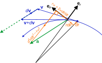
As a generalization of the uniform circular motion case, suppose the angular rate of rotation is not constant. The acceleration now has a tangential component, as shown the image at right. This case is used to demonstrate a derivation strategy based on a polar coordinate system.
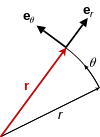
Let r(t) be a vector that describes the position of a point mass as a function of time. Since we are assuming circular motion, let r(t) = R·ur, where R is a constant (the radius of the circle) and ur is the unit vector pointing from the origin to the point mass. The direction of ur is described by θ, the angle between the x-axis and the unit vector, measured counterclockwise from the x-axis. The other unit vector for polar coordinates, uθ is perpendicular to ur and points in the direction of increasing θ. These polar unit vectors can be expressed in terms of Cartesian unit vectors in the x and y directions, denoted and respectively:[17]


One can differentiate to find velocity:

This result for the velocity matches expectations that the velocity should be directed tangentially to the circle, and that the magnitude of the velocity should be rω. Differentiating again, and noting that


Thus, the radial and tangential components of the acceleration are:


These equations express mathematically that, in the case of an object that moves along a circular path with a changing speed, the acceleration of the body may be decomposed into a perpendicular component that changes the direction of motion (the centripetal acceleration), and a parallel, or tangential component, that changes the speed.
General planar motion edit


Polar coordinates edit
The above results can be derived perhaps more simply in polar coordinates, and at the same time extended to general motion within a plane, as shown next. Polar coordinates in the plane employ a radial unit vector uρ and an angular unit vector uθ, as shown above.[18] A particle at position r is described by:

where the notation ρ is used to describe the distance of the path from the origin instead of R to emphasize that this distance is not fixed, but varies with time. The unit vector uρ travels with the particle and always points in the same direction as r(t). Unit vector uθ also travels with the particle and stays orthogonal to uρ. Thus, uρ and uθ form a local Cartesian coordinate system attached to the particle, and tied to the path travelled by the particle.[19] By moving the unit vectors so their tails coincide, as seen in the circle at the left of the image above, it is seen that uρ and uθ form a right-angled pair with tips on the unit circle that trace back and forth on the perimeter of this circle with the same angle θ(t) as r(t).
When the particle moves, its velocity is

To evaluate the velocity, the derivative of the unit vector uρ is needed. Because uρ is a unit vector, its magnitude is fixed, and it can change only in direction, that is, its change duρ has a component only perpendicular to uρ. When the trajectory r(t) rotates an amount dθ, uρ, which points in the same direction as r(t), also rotates by dθ. See image above. Therefore, the change in uρ is

or

In a similar fashion, the rate of change of uθ is found. As with uρ, uθ is a unit vector and can only rotate without changing size. To remain orthogonal to uρ while the trajectory r(t) rotates an amount dθ, uθ, which is orthogonal to r(t), also rotates by dθ. See image above. Therefore, the change duθ is orthogonal to uθ and proportional to dθ (see image above):

The equation above shows the sign to be negative: to maintain orthogonality, if duρ is positive with dθ, then duθ must decrease.
Substituting the derivative of uρ into the expression for velocity:

To obtain the acceleration, another time differentiation is done:

Substituting the derivatives of uρ and uθ, the acceleration of the particle is:[20]
![{\displaystyle {\begin{aligned}\mathbf {a} &={\frac {\mathrm {d} ^{2}\rho }{\mathrm {d} t^{2}}}\mathbf {u} _{\rho }+2{\frac {\mathrm {d} \rho }{\mathrm {d} t}}\mathbf {u} _{\theta }{\frac {\mathrm {d} \theta }{\mathrm {d} t}}-\rho \mathbf {u} _{\rho }\left({\frac {\mathrm {d} \theta }{\mathrm {d} t}}\right)^{2}+\rho \mathbf {u} _{\theta }{\frac {\mathrm {d} ^{2}\theta }{\mathrm {d} t^{2}}}\ ,\\&=\mathbf {u} _{\rho }\left[{\frac {\mathrm {d} ^{2}\rho }{\mathrm {d} t^{2}}}-\rho \left({\frac {\mathrm {d} \theta }{\mathrm {d} t}}\right)^{2}\right]+\mathbf {u} _{\theta }\left[2{\frac {\mathrm {d} \rho }{\mathrm {d} t}}{\frac {\mathrm {d} \theta }{\mathrm {d} t}}+\rho {\frac {\mathrm {d} ^{2}\theta }{\mathrm {d} t^{2}}}\right]\\&=\mathbf {u} _{\rho }\left[{\frac {\mathrm {d} v_{\rho }}{\mathrm {d} t}}-{\frac {v_{\theta }^{2}}{\rho }}\right]+\mathbf {u} _{\theta }\left[{\frac {2}{\rho }}v_{\rho }v_{\theta }+\rho {\frac {\mathrm {d} }{\mathrm {d} t}}{\frac {v_{\theta }}{\rho }}\right]\,.\end{aligned}}}](https://wikimedia.org/api/rest_v1/media/math/render/svg/4bd23fad91b9a145bc62e918b5124ee62c4a537b)
As a particular example, if the particle moves in a circle of constant radius R, then dρ/dt = 0, v = vθ, and:
![{\displaystyle \mathbf {a} =\mathbf {u} _{\rho }\left[-\rho \left({\frac {\mathrm {d} \theta }{\mathrm {d} t}}\right)^{2}\right]+\mathbf {u} _{\theta }\left[\rho {\frac {\mathrm {d} ^{2}\theta }{\mathrm {d} t^{2}}}\right]=\mathbf {u} _{\rho }\left[-{\frac {v^{2}}{r}}\right]+\mathbf {u} _{\theta }\left[{\frac {\mathrm {d} v}{\mathrm {d} t}}\right]\ }](https://wikimedia.org/api/rest_v1/media/math/render/svg/df2f314be17d32d8d204bef757376219863181c7)
where

These results agree with those above for nonuniform circular motion. See also the article on non-uniform circular motion. If this acceleration is multiplied by the particle mass, the leading term is the centripetal force and the negative of the second term related to angular acceleration is sometimes called the Euler force.[21]
For trajectories other than circular motion, for example, the more general trajectory envisioned in the image above, the instantaneous center of rotation and radius of curvature of the trajectory are related only indirectly to the coordinate system defined by uρ and uθ and to the length |r(t)| = ρ. Consequently, in the general case, it is not straightforward to disentangle the centripetal and Euler terms from the above general acceleration equation.[22][23] To deal directly with this issue, local coordinates are preferable, as discussed next.
Local coordinates edit

Local coordinates mean a set of coordinates that travel with the particle,[24] and have orientation determined by the path of the particle.[25] Unit vectors are formed as shown in the image at right, both tangential and normal to the path. This coordinate system sometimes is referred to as intrinsic or path coordinates[26][27] or nt-coordinates, for normal-tangential, referring to these unit vectors. These coordinates are a very special example of a more general concept of local coordinates from the theory of differential forms.[28]
Distance along the path of the particle is the arc length s, considered to be a known function of time.

A center of curvature is defined at each position s located a distance ρ (the radius of curvature) from the curve on a line along the normal un (s). The required distance ρ(s) at arc length s is defined in terms of the rate of rotation of the tangent to the curve, which in turn is determined by the path itself. If the orientation of the tangent relative to some starting position is θ(s), then ρ(s) is defined by the derivative dθ/ds:

The radius of curvature usually is taken as positive (that is, as an absolute value), while the curvature κ is a signed quantity.
A geometric approach to finding the center of curvature and the radius of curvature uses a limiting process leading to the osculating circle.[29][30] See image above.
Using these coordinates, the motion along the path is viewed as a succession of circular paths of ever-changing center, and at each position s constitutes non-uniform circular motion at that position with radius ρ. The local value of the angular rate of rotation then is given by:

with the local speed v given by:

As for the other examples above, because unit vectors cannot change magnitude, their rate of change is always perpendicular to their direction (see the left-hand insert in the image above):[31]


Consequently, the velocity and acceleration are:[30][32][33]

and using the chain-rule of differentiation:
- with the tangential acceleration


In this local coordinate system, the acceleration resembles the expression for nonuniform circular motion with the local radius ρ(s), and the centripetal acceleration is identified as the second term.[34]
Extending this approach to three dimensional space curves leads to the Frenet–Serret formulas.[35][36]
Alternative approach edit
Looking at the image above, one might wonder whether adequate account has been taken of the difference in curvature between ρ(s) and ρ(s + ds) in computing the arc length as ds = ρ(s)dθ. Reassurance on this point can be found using a more formal approach outlined below. This approach also makes connection with the article on curvature.
To introduce the unit vectors of the local coordinate system, one approach is to begin in Cartesian coordinates and describe the local coordinates in terms of these Cartesian coordinates. In terms of arc length s, let the path be described as:[37]
![{\displaystyle \mathbf {r} (s)=\left[x(s),\ y(s)\right].}](https://wikimedia.org/api/rest_v1/media/math/render/svg/ea9cb4aedaa6696cd195a0329b20a3a6d4c1f0d0)
Then an incremental displacement along the path ds is described by:
![{\displaystyle \mathrm {d} \mathbf {r} (s)=\left[\mathrm {d} x(s),\ \mathrm {d} y(s)\right]=\left[x'(s),\ y'(s)\right]\mathrm {d} s\ ,}](https://wikimedia.org/api/rest_v1/media/math/render/svg/6e41305b24920b77bceb3d266edba4ab08249618)
where primes are introduced to denote derivatives with respect to s. The magnitude of this displacement is ds, showing that:[38]
- (Eq. 1)
![{\displaystyle \left[x'(s)^{2}+y'(s)^{2}\right]=1\ .}](https://wikimedia.org/api/rest_v1/media/math/render/svg/50c42e82eda34ce15d98149c930dfb7ba7cec77d)
This displacement is necessarily a tangent to the curve at s, showing that the unit vector tangent to the curve is:
![{\displaystyle \mathbf {u} _{\mathrm {t} }(s)=\left[x'(s),\ y'(s)\right],}](https://wikimedia.org/api/rest_v1/media/math/render/svg/52a7fe41893b23da5d10fa21095cbf823374b339)
![{\displaystyle \mathbf {u} _{\mathrm {n} }(s)=\left[y'(s),\ -x'(s)\right],}](https://wikimedia.org/api/rest_v1/media/math/render/svg/aefd42926b0e6c5fd1cdd0b91ae514b65fd3dfc0)
Orthogonality can be verified by showing that the vector dot product is zero. The unit magnitude of these vectors is a consequence of Eq. 1. Using the tangent vector, the angle θ of the tangent to the curve is given by:


The radius of curvature is introduced completely formally (without need for geometric interpretation) as:

The derivative of θ can be found from that for sinθ:

Now:


![{\displaystyle {\begin{aligned}\mathbf {a} (s)&={\frac {\mathrm {d} }{\mathrm {d} t}}\mathbf {v} (s)={\frac {\mathrm {d} }{\mathrm {d} t}}\left[{\frac {\mathrm {d} s}{\mathrm {d} t}}\left(x'(s),\ y'(s)\right)\right]\\&=\left({\frac {\mathrm {d} ^{2}s}{\mathrm {d} t^{2}}}\right)\mathbf {u} _{\mathrm {t} }(s)+\left({\frac {\mathrm {d} s}{\mathrm {d} t}}\right)^{2}\left(x''(s),\ y''(s)\right)\\&=\left({\frac {\mathrm {d} ^{2}s}{\mathrm {d} t^{2}}}\right)\mathbf {u} _{\mathrm {t} }(s)-\left({\frac {\mathrm {d} s}{\mathrm {d} t}}\right)^{2}{\frac {1}{\rho }}\mathbf {u} _{\mathrm {n} }(s)\end{aligned}}}](https://wikimedia.org/api/rest_v1/media/math/render/svg/c5b63aca630aacb31a8ef0fc21bcf2f8e86af3ca)
This result for acceleration agrees with that found earlier. However, in this approach, the question of the change in radius of curvature with s is handled completely formally, consistent with a geometric interpretation, but not relying upon it, thereby avoiding any questions the image above might suggest about neglecting the variation in ρ.
Example: circular motion edit
To illustrate the above formulas, let x, y be given as:

Then:

which can be recognized as a circular path around the origin with radius α. The position s = 0 corresponds to [α, 0], or 3 o'clock. To use the above formalism, the derivatives are needed:


With these results, one can verify that:

The unit vectors can also be found:
![{\displaystyle \mathbf {u} _{\mathrm {t} }(s)=\left[-\sin {\frac {s}{\alpha }}\ ,\ \cos {\frac {s}{\alpha }}\right]\ ;\ \mathbf {u} _{\mathrm {n} }(s)=\left[\cos {\frac {s}{\alpha }}\ ,\ \sin {\frac {s}{\alpha }}\right]\ ,}](https://wikimedia.org/api/rest_v1/media/math/render/svg/72b1a6646bfe5026f496df581576f09251db1a9c)
which serve to show that s = 0 is located at position [ρ, 0] and s = ρπ/2 at [0, ρ], which agrees with the original expressions for x and y. In other words, s is measured counterclockwise around the circle from 3 o'clock. Also, the derivatives of these vectors can be found:
![{\displaystyle {\frac {\mathrm {d} }{\mathrm {d} s}}\mathbf {u} _{\mathrm {t} }(s)=-{\frac {1}{\alpha }}\left[\cos {\frac {s}{\alpha }}\ ,\ \sin {\frac {s}{\alpha }}\right]=-{\frac {1}{\alpha }}\mathbf {u} _{\mathrm {n} }(s)\ ;}](https://wikimedia.org/api/rest_v1/media/math/render/svg/0d6d3efccbed76c27507654645897ccc0b587b08)
![{\displaystyle \ {\frac {\mathrm {d} }{\mathrm {d} s}}\mathbf {u} _{\mathrm {n} }(s)={\frac {1}{\alpha }}\left[-\sin {\frac {s}{\alpha }}\ ,\ \cos {\frac {s}{\alpha }}\right]={\frac {1}{\alpha }}\mathbf {u} _{\mathrm {t} }(s)\ .}](https://wikimedia.org/api/rest_v1/media/math/render/svg/29f755d9d1bb8f6f884a3bdc8ae8d1be5147674a)
To obtain velocity and acceleration, a time-dependence for s is necessary. For counterclockwise motion at variable speed v(t):

where v(t) is the speed and t is time, and s(t = 0) = 0. Then:


where it already is established that α = ρ. This acceleration is the standard result for non-uniform circular motion.
See also edit
- Analytical mechanics
- Applied mechanics
- Bertrand theorem
- Central force
- Centrifugal force
- Circular motion
- Classical mechanics
- Coriolis force
- Dynamics (physics)
- Eskimo yo-yo
- Example: circular motion
- Fictitious force
- Frenet-Serret formulas
- History of centrifugal and centripetal forces
- Kinematics
- Kinetics
- Mechanics of planar particle motion
- Orthogonal coordinates
- Reactive centrifugal force
- Statics
Notes and references edit
- ^ Craig, John (1849). A new universal etymological, technological and pronouncing dictionary of the English language: embracing all terms used in art, science, and literature, Volume 1. Harvard University. p. 291. Extract of page 291
- ^ Newton, Isaac (2010). The principia : mathematical principles of natural philosophy. [S.l.]: Snowball Pub. p. 10. ISBN 978-1-60796-240-3.
- ^ Russelkl C Hibbeler (2009). "Equations of Motion: Normal and tangential coordinates". Engineering Mechanics: Dynamics (12 ed.). Prentice Hall. p. 131. ISBN 978-0-13-607791-6.
- ^ Paul Allen Tipler; Gene Mosca (2003). Physics for scientists and engineers (5th ed.). Macmillan. p. 129. ISBN 978-0-7167-8339-8.
- ^ P. Germain; M. Piau; D. Caillerie, eds. (2012). Theoretical and Applied Mechanics. Elsevier. ISBN 9780444600202.
- ^ Chris Carter (2001). Facts and Practice for A-Level: Physics. S.2.: Oxford University Press. p. 30. ISBN 978-0-19-914768-7.
{{cite book}}: CS1 maint: location (link) - ^ a b OpenStax CNX. "Uniform Circular Motion".
- ^ Eugene Lommel; George William Myers (1900). Experimental physics. K. Paul, Trench, Trübner & Co. p. 63.
- ^ Colwell, Catharine H. "A Derivation of the Formulas for Centripetal Acceleration". PhysicsLAB. Archived from the original on 15 August 2011. Retrieved 31 July 2011.
- ^ Conte, Mario; Mackay, William W (1991). An Introduction to the Physics of Particle Accelerators. World Scientific. p. 8. ISBN 978-981-4518-00-0. Extract of page 8
- ^ Theo Koupelis (2010). In Quest of the Universe (6th ed.). Jones & Bartlett Learning. p. 83. ISBN 978-0-7637-6858-4.
- ^ A. V. Durrant (1996). Vectors in physics and engineering. CRC Press. p. 103. ISBN 978-0-412-62710-1.
- ^ Lawrence S. Lerner (1997). Physics for Scientists and Engineers. Boston: Jones & Bartlett Publishers. p. 128. ISBN 978-0-86720-479-7.
- ^ Arthur Beiser (2004). Schaum's Outline of Applied Physics. New York: McGraw-Hill Professional. p. 103. ISBN 978-0-07-142611-4.
- ^ Alan Darbyshire (2003). Mechanical Engineering: BTEC National Option Units. Oxford: Newnes. p. 56. ISBN 978-0-7506-5761-7.
- ^ Federal Aviation Administration (2007). Pilot's Encyclopedia of Aeronautical Knowledge. Oklahoma City OK: Skyhorse Publishing Inc. Figure 3–21. ISBN 978-1-60239-034-8.
- ^ Note: unlike the Cartesian unit vectors and , which are constant, in polar coordinates the direction of the unit vectors ur and uθ depend on θ, and so in general have non-zero time derivatives.
- ^ Although the polar coordinate system moves with the particle, the observer does not. The description of the particle motion remains a description from the stationary observer's point of view.
- ^ Notice that this local coordinate system is not autonomous; for example, its rotation in time is dictated by the trajectory traced by the particle. The radial vector r(t) does not represent the radius of curvature of the path.
- ^ John Robert Taylor (2005). Classical Mechanics. Sausalito CA: University Science Books. pp. 28–29. ISBN 978-1-891389-22-1.
- ^ Cornelius Lanczos (1986). The Variational Principles of Mechanics. New York: Courier Dover Publications. p. 103. ISBN 978-0-486-65067-8.
- ^ See, for example, Howard D. Curtis (2005). Orbital Mechanics for Engineering Students. Butterworth-Heinemann. p. 5. ISBN 978-0-7506-6169-0.
- ^ S. Y. Lee (2004). Accelerator physics (2nd ed.). Hackensack NJ: World Scientific. p. 37. ISBN 978-981-256-182-4.
- ^ The observer of the motion along the curve is using these local coordinates to describe the motion from the observer's frame of reference, that is, from a stationary point of view. In other words, although the local coordinate system moves with the particle, the observer does not. A change in coordinate system used by the observer is only a change in their description of observations, and does not mean that the observer has changed their state of motion, and vice versa.
- ^ Zhilin Li; Kazufumi Ito (2006). The immersed interface method: numerical solutions of PDEs involving interfaces and irregular domains. Philadelphia: Society for Industrial and Applied Mathematics. p. 16. ISBN 978-0-89871-609-2.
- ^ K L Kumar (2003). Engineering Mechanics. New Delhi: Tata McGraw-Hill. p. 339. ISBN 978-0-07-049473-2.
- ^ Lakshmana C. Rao; J. Lakshminarasimhan; Raju Sethuraman; SM Sivakuma (2004). Engineering Dynamics: Statics and Dynamics. Prentice Hall of India. p. 133. ISBN 978-81-203-2189-2.
- ^ Shigeyuki Morita (2001). Geometry of Differential Forms. American Mathematical Society. p. 1. ISBN 978-0-8218-1045-3.
local coordinates.
- ^ The osculating circle at a given point P on a curve is the limiting circle of a sequence of circles that pass through P and two other points on the curve, Q and R, on either side of P, as Q and R approach P. See the online text by Lamb: Horace Lamb (1897). An Elementary Course of Infinitesimal Calculus. University Press. p. 406. ISBN 978-1-108-00534-0.
osculating circle.
- ^ a b Guang Chen; Fook Fah Yap (2003). An Introduction to Planar Dynamics (3rd ed.). Central Learning Asia/Thomson Learning Asia. p. 34. ISBN 978-981-243-568-2.
- ^ R. Douglas Gregory (2006). Classical Mechanics: An Undergraduate Text. Cambridge University Press. p. 20. ISBN 978-0-521-82678-5.
- ^ Edmund Taylor Whittaker; William McCrea (1988). A Treatise on the Analytical Dynamics of Particles and Rigid Bodies: with an introduction to the problem of three bodies (4th ed.). Cambridge University Press. p. 20. ISBN 978-0-521-35883-5.
- ^ Jerry H. Ginsberg (2007). Engineering Dynamics. Cambridge University Press. p. 33. ISBN 978-0-521-88303-0.
- ^ Joseph F. Shelley (1990). 800 solved problems in vector mechanics for engineers: Dynamics. McGraw-Hill Professional. p. 47. ISBN 978-0-07-056687-3.
- ^ Larry C. Andrews; Ronald L. Phillips (2003). Mathematical Techniques for Engineers and Scientists. SPIE Press. p. 164. ISBN 978-0-8194-4506-3.
- ^ Ch V Ramana Murthy; NC Srinivas (2001). Applied Mathematics. New Delhi: S. Chand & Co. p. 337. ISBN 978-81-219-2082-7.
- ^ The article on curvature treats a more general case where the curve is parametrized by an arbitrary variable (denoted t), rather than by the arc length s.
- ^ Ahmed A. Shabana; Khaled E. Zaazaa; Hiroyuki Sugiyama (2007). Railroad Vehicle Dynamics: A Computational Approach. CRC Press. p. 91. ISBN 978-1-4200-4581-9.
Further reading edit
- Serway, Raymond A.; Jewett, John W. (2004). Physics for Scientists and Engineers (6th ed.). Brooks/Cole. ISBN 978-0-534-40842-8.
- Tipler, Paul (2004). Physics for Scientists and Engineers: Mechanics, Oscillations and Waves, Thermodynamics (5th ed.). W. H. Freeman. ISBN 978-0-7167-0809-4.
- Centripetal force vs. Centrifugal force, from an online Regents Exam physics tutorial by the Oswego City School District
External links edit
- Notes from Physics and Astronomy HyperPhysics at Georgia State University