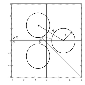
An excellent example system is the "Gaspard–Rice" (GR) scattering system ^[1] —also known simply as the "three-disc" system—which embodies many of the important concepts in chaotic scattering while being simple and easy to understand and simulate. The concept is very simple: we have three hard discs arranged in some triangular formation, a point particle is sent in and undergoes perfect, elastic collisions until it exits towards infinity. In this discussion, we will only consider GR systems having equally sized discs, equally spaced around the points of an equilateral triangle.

Figure 1 illustrates this system while Figure 2 shows two example trajectories. Note first that the trajectories bounce around the system for some time before finally exiting. Note also, that if we consider the impact parameters to be the start of the two perfectly horizontal lines at left (the system is completely reversible: the exit point could also be the entry point), the two trajectories are initially so close as to be almost identical. By the time they exit, they are completely different, thus illustrating the strong sensitivity to initial conditions. This system will be used as an example throughout the article.

If we introduce a large number of particles with uniformly distributed impact parameters, the rate at which they exit the system is known as the decay rate. We can calculate the decay rate by simulating the system over many trials and forming a histogram of the delay time, T. For the GR system, it is easy to see that the delay time and the length of the particle trajectory are equivalent but for a multiplication coefficient. A typical choice for the impact parameter is the y-coordinate, while the trajectory angle is kept constant at zero degrees—horizontal. Meanwhile, we say that the particle has "exited the system" once it passes a border some arbitrary, but sufficiently large, distance from the centre of the system.

We expect the number of particles remaining in the system, N(T), to vary as:

${\displaystyle N(T)\sim e^{-\gamma T}}$ 

Thus the decay rate, ${\displaystyle \gamma }$ , is given as:

${\displaystyle \gamma =\lim _{n\rightarrow \infty }-{\frac {\ln N(T)}{T}}}$ 

where n is the total number of particles. ^[2]

Figure 3 shows a plot of the path-length versus the number of particles for a simulation of one million (1e6) particles started with random impact parameter, b. A fitted straight line of negative slope, ${\displaystyle \gamma =0.739}$  is overlaid. The path-length, s, is equivalent to the decay time, T, provided we scale the (constant) speed appropriately. Note that an exponential decay rate is a property specifically of hyperbolic chaotic scattering. Non-hyperbolic scatterers may have an arithmetic decay rate. ^[3]

Figure 4 shows an experimental realization of the Gaspard–Rice system using a laser instead of a point particle. As anyone who's actually tried this knows, this is not a very effective method of testing the system—the laser beam gets scattered in every direction. As shown by Sweet, Ott and Yorke, ^[5] a more effective method is to direct coloured light through the gaps between the discs (or in this case, tape coloured strips of paper across pairs of cylinders) and view the reflections through an open gap. The result is a complex pattern of stripes of alternating colour, as shown below, seen more clearly in the simulated version below that.

Figures 5 and 6 show the basins of attraction for each impact parameter, b, that is, for a given value of b, through which gap does the particle exit? The basin boundaries form a Cantor set and represent members of the stable manifold: trajectories that, once started, never exit the system.

So long as it is symmetric, we can easily think of the system as an iterated function map, a common method of representing a chaotic, dynamical system. ^[7] Figure 7 shows one possible representation of the variables, with the first variable, ${\displaystyle \theta \in [-\pi ,\pi ]}$ , representing the angle around the disc at rebound and the second, ${\displaystyle \phi \in [-\pi /2,\pi /2]}$ , representing the impact/rebound angle relative to the disc. A subset of these two variables, called the invariant set will map onto themselves. This set, four members of which are shown in Figures 8 and 9, will be fractal, totally non-attracting and of measure zero. This is an interesting inversion of the more normally discussed chaotic systems in which the fractal invariant set is attracting and in fact comprises the basin[s] of attraction. Note that the totally non-attracting nature of the invariant set is another property of a hyperbolic chaotic scatterer.

Each member of the invariant set can be modelled using symbolic dynamics: the trajectory is labelled based on each of the discs off of which it rebounds. The set of all such sequences form an uncountable set.^[8] For the four members shown in Figures 8 and 9, the symbolic dynamics will be as follows: ^[3]

...121212121212...
...232323232323...
...313131313131...
...123123123123...

Members of the stable manifold may be likewise represented, except each sequence will have a starting point. When you consider that a member of the invariant set must "fit" in the boundaries between two basins of attraction, it is apparent that, if perturbed, the trajectory may exit anywhere along the sequence. Thus it should also be apparent that an infinite number of alternating basins of all three "colours" will exist between any given boundary. ^[2][3][8]

Because of their unstable nature, it is difficult to access members of the invariant set or the stable manifold directly. The uncertainty exponent is ideally tailored to measure the fractal dimension of this type of system. Once again using the single impact parameter, b, we perform multiple trials with random impact parameters, perturbing them by a minute amount, ${\displaystyle \epsilon }$ , and counting how frequently the number of rebounds off the discs changes, that is, the uncertainty fraction. Note that even though the system is two dimensional, a single impact parameter is sufficient to measure the fractal dimension of the stable manifold. This is demonstrated in Figure 10, which shows the basins of attraction plotted as a function of a dual impact parameter, ${\displaystyle \theta }$  and ${\displaystyle \phi }$ . The stable manifold, which can be seen in the boundaries between the basins, is fractal along only one dimension.

Figure 11 plots the uncertainty fraction, f, as a function of the uncertainty, ${\displaystyle \epsilon }$  for a simulated Gaspard–Rice system. The slope of the fitted curve returns the uncertainty exponent, ${\displaystyle \gamma =0.380}$ , thus the box-counting dimension of the stable manifold is, ${\displaystyle D_{0}=N-\gamma =2-0.380=1.62}$ . The invariant set is the intersection of the stable and unstable manifolds. ^[9]

Since the system is the same whether run forwards or backwards, the unstable manifold is simply the mirror image of the stable manifold and their fractal dimensions will be equal. ^[8] On this basis we can calculate the fractal dimension of the invariant set:^[2]

${\displaystyle D=D_{s}+D_{u}-N=2D_{s}-N=N-2\gamma }$ 

where D_s and D_u are the fractal dimensions of the stable and unstable manifolds, respectively and N=2 is the dimensionality of the system. The fractal dimension of the invariant set is D=1.24.

From the preceding discussion, it should be apparent that the decay rate, the fractal dimension and the Lyapunov exponents are all related. The large Lyapunov exponent, for instance, tells us how fast a trajectory in the invariant set will diverge if perturbed. Similarly, the fractal dimension will give us information about the density of orbits in the invariant set. Thus we can see that both will affect the decay rate as captured in the following conjecture for a two-dimensional scattering system:^[2]

${\displaystyle D_{1}=\left(h_{1}-{\frac {1}{\gamma }}\right)\left({\frac {1}{h_{1}}}-{\frac {1}{h_{2}}}\right)}$ 

where D₁ is the information dimension and h₁ and h₂ are the small and large Lyapunov exponents, respectively. For an attractor, ${\displaystyle \gamma =\infty }$  and it reduces to the Kaplan–Yorke conjecture.^[2]

• Lakes of Wada
• Uncertainty exponent

• Software for simulating the Gaspard–Rice system
• A simulation of the Gaspard-Rice system's and its symbolic dynamics, from Chaos V: Duhem's Bull