


Summary
In computational complexity theory, a complexity class is a set of computational problems "of related resource-based complexity".[1] The two most commonly analyzed resources are time and memory.
In general, a complexity class is defined in terms of a type of computational problem, a model of computation, and a bounded resource like time or memory. In particular, most complexity classes consist of decision problems that are solvable with a Turing machine, and are differentiated by their time or space (memory) requirements. For instance, the class P is the set of decision problems solvable by a deterministic Turing machine in polynomial time. There are, however, many complexity classes defined in terms of other types of problems (e.g. counting problems and function problems) and using other models of computation (e.g. probabilistic Turing machines, interactive proof systems, Boolean circuits, and quantum computers).
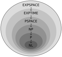
The study of the relationships between complexity classes is a major area of research in theoretical computer science. There are often general hierarchies of complexity classes; for example, it is known that a number of fundamental time and space complexity classes relate to each other in the following way: L⊆NL⊆P⊆NP⊆PSPACE⊆EXPTIME⊆NEXPTIME⊆EXPSPACE (where ⊆ denotes the subset relation). However, many relationships are not yet known; for example, one of the most famous open problems in computer science concerns whether P equals NP. The relationships between classes often answer questions about the fundamental nature of computation. The P versus NP problem, for instance, is directly related to questions of whether nondeterminism adds any computational power to computers and whether problems having solutions that can be quickly checked for correctness can also be quickly solved.
Background edit
Complexity classes are sets of related computational problems. They are defined in terms of the computational difficulty of solving the problems contained within them with respect to particular computational resources like time or memory. More formally, the definition of a complexity class consists of three things: a type of computational problem, a model of computation, and a bounded computational resource. In particular, most complexity classes consist of decision problems that can be solved by a Turing machine with bounded time or space resources. For example, the complexity class P is defined as the set of decision problems that can be solved by a deterministic Turing machine in polynomial time.
Computational problems edit
Intuitively, a computational problem is just a question that can be solved by an algorithm. For example, "is the natural number prime?" is a computational problem. A computational problem is mathematically represented as the set of answers to the problem. In the primality example, the problem (call it ) is represented by the set of all natural numbers that are prime: . In the theory of computation, these answers are represented as strings; for example, in the primality example the natural numbers could be represented as strings of bits that represent binary numbers. For this reason, computational problems are often synonymously referred to as languages, since strings of bits represent formal languages (a concept borrowed from linguistics); for example, saying that the problem is in the complexity class NP is equivalent to saying that the language is in NP.


Decision problems edit

The most commonly analyzed problems in theoretical computer science are decision problems—the kinds of problems that can be posed as yes–no questions. The primality example above, for instance, is an example of a decision problem as it can be represented by the yes–no question "is the natural number prime". In terms of the theory of computation, a decision problem is represented as the set of input strings that a computer running a correct algorithm would answer "yes" to. In the primality example, is the set of strings representing natural numbers that, when input into a computer running an algorithm that correctly tests for primality, the algorithm answers "yes, this number is prime". This "yes-no" format is often equivalently stated as "accept-reject"; that is, an algorithm "accepts" an input string if the answer to the decision problem is "yes" and "rejects" if the answer is "no".
While some problems cannot easily be expressed as decision problems, they nonetheless encompass a broad range of computational problems.[2] Other types of problems that certain complexity classes are defined in terms of include function problems (e.g. FP), counting problems (e.g. #P), optimization problems, and promise problems (see section "Other types of problems").
Computational models edit
To make concrete the notion of a "computer", in theoretical computer science problems are analyzed in the context of a computational model. Computational models make exact the notions of computational resources like "time" and "memory". In computational complexity theory, complexity classes deal with the inherent resource requirements of problems and not the resource requirements that depend upon how a physical computer is constructed. For example, in the real world different computers may require different amounts of time and memory to solve the same problem because of the way that they have been engineered. By providing an abstract mathematical representations of computers, computational models abstract away superfluous complexities of the real world (like differences in processor speed) that obstruct an understanding of fundamental principles.
The most commonly used computational model is the Turing machine. While other models exist and many complexity classes are defined in terms of them (see section "Other models of computation"), the Turing machine is used to define most basic complexity classes. With the Turing machine, instead of using standard units of time like the second (which make it impossible to disentangle running time from the speed of physical hardware) and standard units of memory like bytes, the notion of time is abstracted as the number of elementary steps that a Turing machine takes to solve a problem and the notion of memory is abstracted as the number of cells that are used on the machine's tape. These are explained in greater detail below.
It is also possible to use the Blum axioms to define complexity classes without referring to a concrete computational model, but this approach is less frequently used in complexity theory.
Deterministic Turing machines edit

A Turing machine is a mathematical model of a general computing machine. It is the most commonly used model in complexity theory, owing in large part to the fact that it is believed to be as powerful as any other model of computation and is easy to analyze mathematically. Importantly, it is believed that if there exists an algorithm that solves a particular problem then there also exists a Turing machine that solves that same problem (this is known as the Church–Turing thesis); this means that it is believed that every algorithm can be represented as a Turing machine.
Mechanically, a Turing machine (TM) manipulates symbols (generally restricted to the bits 0 and 1 to provide an intuitive connection to real-life computers) contained on an infinitely long strip of tape. The TM can read and write, one at a time, using a tape head. Operation is fully determined by a finite set of elementary instructions such as "in state 42, if the symbol seen is 0, write a 1; if the symbol seen is 1, change into state 17; in state 17, if the symbol seen is 0, write a 1 and change to state 6". The Turing machine starts with only the input string on its tape and blanks everywhere else. The TM accepts the input if it enters a designated accept state and rejects the input if it enters a reject state. The deterministic Turing machine (DTM) is the most basic type of Turing machine. It uses a fixed set of rules to determine its future actions (which is why it is called "deterministic").
A computational problem can then be defined in terms of a Turing machine as the set of input strings that a particular Turing machine accepts. For example, the primality problem from above is the set of strings (representing natural numbers) that a Turing machine running an algorithm that correctly tests for primality accepts. A Turing machine is said to recognize a language (recall that "problem" and "language" are largely synonymous in computability and complexity theory) if it accepts all inputs that are in the language and is said to decide a language if it additionally rejects all inputs that are not in the language (certain inputs may cause a Turing machine to run forever, so decidability places the additional constraint over recognizability that the Turing machine must halt on all inputs). A Turing machine that "solves" a problem is generally meant to mean one that decides the language.
Turing machines enable intuitive notions of "time" and "space". The time complexity of a TM on a particular input is the number of elementary steps that the Turing machine takes to reach either an accept or reject state. The space complexity is the number of cells on its tape that it uses to reach either an accept or reject state.
Nondeterministic Turing machines edit

The deterministic Turing machine (DTM) is a variant of the nondeterministic Turing machine (NTM). Intuitively, an NTM is just a regular Turing machine that has the added capability of being able to explore multiple possible future actions from a given state, and "choosing" a branch that accepts (if any accept). That is, while a DTM must follow only one branch of computation, an NTM can be imagined as a computation tree, branching into many possible computational pathways at each step (see image). If at least one branch of the tree halts with an "accept" condition, then the NTM accepts the input. In this way, an NTM can be thought of as simultaneously exploring all computational possibilities in parallel and selecting an accepting branch.[3] NTMs are not meant to be physically realizable models, they are simply theoretically interesting abstract machines that give rise to a number of interesting complexity classes (which often do have physically realizable equivalent definitions).
The time complexity of an NTM is the maximum number of steps that the NTM uses on any branch of its computation.[4] Similarly, the space complexity of an NTM is the maximum number of cells that the NTM uses on any branch of its computation.
DTMs can be viewed as a special case of NTMs that do not make use of the power of nondeterminism. Hence, every computation that can be carried out by a DTM can also be carried out by an equivalent NTM. It is also possible to simulate any NTM using a DTM (the DTM will simply compute every possible computational branch one-by-one). Hence, the two are equivalent in terms of computability. However, simulating an NTM with a DTM often requires greater time and/or memory resources; as will be seen, how significant this slowdown is for certain classes of computational problems is an important question in computational complexity theory.
Resource bounds edit
Complexity classes group computational problems by their resource requirements. To do this, computational problems are differentiated by upper bounds on the maximum amount of resources that the most efficient algorithm takes to solve them. More specifically, complexity classes are concerned with the rate of growth in the resources required to solve particular computational problems as the input size increases. For example, the amount of time it takes to solve problems in the complexity class P grows at a polynomial rate as the input size increases, which is comparatively slow compared to problems in the exponential complexity class EXPTIME (or more accurately, for problems in EXPTIME that are outside of P, since ).

Note that the study of complexity classes is intended primarily to understand the inherent complexity required to solve computational problems. Complexity theorists are thus generally concerned with finding the smallest complexity class that a problem falls into and are therefore concerned with identifying which class a computational problem falls into using the most efficient algorithm. There may be an algorithm, for instance, that solves a particular problem in exponential time, but if the most efficient algorithm for solving this problem runs in polynomial time then the inherent time complexity of that problem is better described as polynomial.
Time bounds edit
The time complexity of an algorithm with respect to the Turing machine model is the number of steps it takes for a Turing machine to run an algorithm on a given input size. Formally, the time complexity for an algorithm implemented with a Turing machine is defined as the function , where is the maximum number of steps that takes on any input of length .


In computational complexity theory, theoretical computer scientists are concerned less with particular runtime values and more with the general class of functions that the time complexity function falls into. For instance, is the time complexity function a polynomial? A logarithmic function? An exponential function? Or another kind of function?
Space bounds edit
The space complexity of an algorithm with respect to the Turing machine model is the number of cells on the Turing machine's tape that are required to run an algorithm on a given input size. Formally, the space complexity of an algorithm implemented with a Turing machine is defined as the function , where is the maximum number of cells that uses on any input of length .


Basic complexity classes edit
Basic definitions edit
Complexity classes are often defined using granular sets of complexity classes called DTIME and NTIME (for time complexity) and DSPACE and NSPACE (for space complexity). Using big O notation, they are defined as follows:
- The time complexity class is the set of all problems that are decided by an time deterministic Turing machine.
- The time complexity class is the set of all problems that are decided by an time nondeterministic Turing machine.
- The space complexity class is the set of all problems that are decided by an space deterministic Turing machine.
- The space complexity class is the set of all problems that are decided by an space nondeterministic Turing machine.


Time complexity classes edit
P and NP edit
P is the class of problems that are solvable by a deterministic Turing machine in polynomial time and NP is the class of problems that are solvable by a nondeterministic Turing machine in polynomial time. Or more formally,


P is often said to be the class of problems that can be solved "quickly" or "efficiently" by a deterministic computer, since the time complexity of solving a problem in P increases relatively slowly with the input size.
An important characteristic of the class NP is that it can be equivalently defined as the class of problems whose solutions are verifiable by a deterministic Turing machine in polynomial time. That is, a language is in NP if there exists a deterministic polynomial time Turing machine, referred to as the verifier, that takes as input a string and a polynomial-size certificate string , and accepts if is in the language and rejects if is not in the language. Intuitively, the certificate acts as a proof that the input is in the language. Formally:[5]


- NP is the class of languages for which there exists a polynomial-time deterministic Turing machine and a polynomial such that for all , is in if and only if there exists some such that accepts.


This equivalence between the nondeterministic definition and the verifier definition highlights a fundamental connection between nondeterminism and solution verifiability. Furthermore, it also provides a useful method for proving that a language is in NP—simply identify a suitable certificate and show that it can be verified in polynomial time.
The P versus NP problem edit
While there might seem to be an obvious difference between the class of problems that are efficiently solvable and the class of problems whose solutions are merely efficiently checkable, P and NP are actually at the center of one of the most famous unsolved problems in computer science: the P versus NP problem. While it is known that P NP (intuitively, deterministic Turing machines are just a subclass of nondeterministic Turing machines that don't make use of their nondeterminism; or under the verifier definition, P is the class of problems whose polynomial time verifiers need only receive the empty string as their certificate), it is not known whether NP is strictly larger than P. If P=NP, then it follows that nondeterminism provides no additional computational power over determinism with regards to the ability to quickly find a solution to a problem; that is, being able to explore all possible branches of computation provides at most a polynomial speedup over being able to explore only a single branch. Furthermore, it would follow that if there exists a proof for a problem instance and that proof can be quickly be checked for correctness (that is, if the problem is in NP), then there also exists an algorithm that can quickly construct that proof (that is, the problem is in P).[6] However, the overwhelming majority of computer scientists believe that P NP,[7] and most cryptographic schemes employed today rely on the assumption that P NP.[8]


EXPTIME and NEXPTIME edit
EXPTIME (sometimes shortened to EXP) is the class of decision problems solvable by a deterministic Turing machine in exponential time and NEXPTIME (sometimes shortened to NEXP) is the class of decision problems solvable by a nondeterministic Turing machine in exponential time. Or more formally,


EXPTIME is a strict superset of P and NEXPTIME is a strict superset of NP. It is further the case that EXPTIME NEXPTIME. It is not known whether this is proper, but if P=NP then EXPTIME must equal NEXPTIME.
Space complexity classes edit
L and NL edit
While it is possible to define logarithmic time complexity classes, these are extremely narrow classes as sublinear times do not even enable a Turing machine to read the entire input (because ).[a][9] However, there are a meaningful number of problems that can be solved in logarithmic space. The definitions of these classes require a two-tape Turing machine so that it is possible for the machine to store the entire input (it can be shown that in terms of computability the two-tape Turing machine is equivalent to the single-tape Turing machine).[10] In the two-tape Turing machine model, one tape is the input tape, which is read-only. The other is the work tape, which allows both reading and writing and is the tape on which the Turing machine performs computations. The space complexity of the Turing machine is measured as the number of cells that are used on the work tape.

L (sometimes lengthened to LOGSPACE) is then defined as the class of problems solvable in logarithmic space on a deterministic Turing machine and NL (sometimes lengthened to NLOGSPACE) is the class of problems solvable in logarithmic space on a nondeterministic Turing machine. Or more formally,[10]


It is known that . However, it is not known whether any of these relationships is proper.

PSPACE and NPSPACE edit
The complexity classes PSPACE and NPSPACE are the space analogues to P and NP. That is, PSPACE is the class of problems solvable in polynomial space by a deterministic Turing machine and NPSPACE is the class of problems solvable in polynomial space by a nondeterministic Turing machine. More formally,


While it is not known whether P=NP, Savitch's theorem famously showed that PSPACE=NPSPACE. It is also known that P PSPACE, which follows intuitively from the fact that, since writing to a cell on a Turing machine's tape is defined as taking one unit of time, a Turing machine operating in polynomial time can only write to polynomially many cells. It is suspected that P is strictly smaller than PSPACE, but this has not been proven.
EXPSPACE and NEXPSPACE edit
The complexity classes EXPSPACE and NEXPSPACE are the space analogues to EXPTIME and NEXPTIME. That is, EXPSPACE is the class of problems solvable in exponential space by a deterministic Turing machine and NEXPSPACE is the class of problems solvable in exponential space by a nondeterministic Turing machine. Or more formally,


Savitch's theorem showed that EXPSPACE=NEXPSPACE. This class is extremely broad: it is known to be a strict superset of PSPACE, NP, and P, and is believed to be a strict superset of EXPTIME.
Properties of complexity classes edit
Closure edit
Complexity classes have a variety of closure properties. For example, decision classes may be closed under negation, disjunction, conjunction, or even under all Boolean operations. Moreover, they might also be closed under a variety of quantification schemes. P, for instance, is closed under all Boolean operations, and under quantification over polynomially sized domains. Closure properties can be helpful in separating classes—one possible route to separating two complexity classes is to find some closure property possessed by one class but not by the other.
Each class X that is not closed under negation has a complement class co-X, which consists of the complements of the languages contained in X (i.e. co-X= X ). co-NP, for instance, is one important complement complexity class, and sits at the center of the unsolved problem over whether co-NP=NP.


Closure properties are one of the key reasons many complexity classes are defined in the way that they are.[11] Take, for example, a problem that can be solved in time (that is, in linear time) and one that can be solved in, at best, time. Both of these problems are in P, yet the runtime of the second grows considerably faster than the runtime of the first as the input size increases. One might ask whether it would be better to define the class of "efficiently solvable" problems using some smaller polynomial bound, like , rather than all polynomials, which allows for such large discrepancies. It turns out, however, that the set of all polynomials is the smallest class of functions containing the linear functions that is also closed under addition, multiplication, and composition (for instance, , which is a polynomial but ).[11] Since we would like composing one efficient algorithm with another efficient algorithm to still be considered efficient, the polynomials are the smallest class that ensures composition of "efficient algorithms".[12] (Note that the definition of P is also useful because, empirically, almost all problems in P that are practically useful do in fact have low order polynomial runtimes, and almost all problems outside of P that are practically useful do not have any known algorithms with small exponential runtimes, i.e. with runtimes where is close to 1.[13])


Reductions edit
Many complexity classes are defined using the concept of a reduction. A reduction is a transformation of one problem into another problem, i.e. a reduction takes inputs from one problem and transforms them into inputs of another problem. For instance, you can reduce ordinary base-10 addition to base-2 addition by transforming and to their base-2 notation (e.g. 5+7 becomes 101+111). Formally, a problem reduces to a problem if there exists a function such that for every , if and only if .


Generally, reductions are used to capture the notion of a problem being at least as difficult as another problem. Thus we are generally interested in using a polynomial-time reduction, since any problem that can be efficiently reduced to another problem is no more difficult than . Formally, a problem is polynomial-time reducible to a problem if there exists a polynomial-time computable function such that for all , if and only if .

Note that reductions can be defined in many different ways. Common reductions are Cook reductions, Karp reductions and Levin reductions, and can vary based on resource bounds, such as polynomial-time reductions and log-space reductions.
Hardness edit
Reductions motivate the concept of a problem being hard for a complexity class. A problem is hard for a class of problems C if every problem in C can be polynomial-time reduced to . Thus no problem in C is harder than , since an algorithm for allows us to solve any problem in C with at most polynomial slowdown. Of particular importance, the set of problems that are hard for NP is called the set of NP-hard problems.
Completeness edit
If a problem is hard for C and is also in C, then is said to be complete for C. This means that is the hardest problem in C (since there could be many problems that are equally hard, more precisely is as hard as the hardest problems in C).
Of particular importance is the class of NP-complete problems—the most difficult problems in NP. Because all problems in NP can be polynomial-time reduced to NP-complete problems, finding an NP-complete problem that can be solved in polynomial time would mean that P = NP.
Relationships between complexity classes edit
Savitch's theorem edit
Savitch's theorem establishes the relationship between deterministic and nondetermistic space resources. It shows that if a nondeterministic Turing machine can solve a problem using space, then a deterministic Turing machine can solve the same problem in space, i.e. in the square of the space. Formally, Savitch's theorem states that for any ,[14]


Important corollaries of Savitch's theorem are that PSPACE = NPSPACE (since the square of a polynomial is still a polynomial) and EXPSPACE = NEXPSPACE (since the square of an exponential is still an exponential).
These relationships answer fundamental questions about the power of nondeterminism compared to determinism. Specifically, Savitch's theorem shows that any problem that a nondeterministic Turing machine can solve in polynomial space, a deterministic Turing machine can also solve in polynomial space. Similarly, any problem that a nondeterministic Turing machine can solve in exponential space, a deterministic Turing machine can also solve in exponential space.
Hierarchy theorems edit
By definition of DTIME, it follows that is contained in if , since if . However, this definition gives no indication of whether this inclusion is strict. For time and space requirements, the conditions under which the inclusion is strict are given by the time and space hierarchy theorems, respectively. They are called hierarchy theorems because they induce a proper hierarchy on the classes defined by constraining the respective resources. The hierarchy theorems enable one to make quantitative statements about how much more additional time or space is needed in order to increase the number of problems that can be solved.


The time hierarchy theorem states that
- .

The space hierarchy theorem states that
- .

The time and space hierarchy theorems form the basis for most separation results of complexity classes. For instance, the time hierarchy theorem establishes that P is strictly contained in EXPTIME, and the space hierarchy theorem establishes that L is strictly contained in PSPACE.
Other models of computation edit
While deterministic and non-deterministic Turing machines are the most commonly used models of computation, many complexity classes are defined in terms of other computational models. In particular,
- A number of classes are defined using probabilistic Turing machines, including the classes BPP, PP, RP, and ZPP
- A number of classes are defined using interactive proof systems, including the classes IP, MA, and AM
- A number of classes are defined using Boolean circuits, including the classes P/poly and its subclasses NC and AC
- A number of classes are defined using quantum Turing machines, including the classes BQP and QMA
These are explained in greater detail below.
Randomized computation edit
A number of important complexity classes are defined using the probabilistic Turing machine, a variant of the Turing machine that can toss random coins. These classes help to better describe the complexity of randomized algorithms.
A probabilistic Turing machine is similar to a deterministic Turing machine, except rather than following a single transition function (a set of rules for how to proceed at each step of the computation) it probabilistically selects between multiple transition functions at each step. The standard definition of a probabilistic Turing machine specifies two transition functions, so that the selection of transition function at each step resembles a coin flip. The randomness introduced at each step of the computation introduces the potential for error; that is, strings that the Turing machine is meant to accept may on some occasions be rejected and strings that the Turing machine is meant to reject may on some occasions be accepted. As a result, the complexity classes based on the probabilistic Turing machine are defined in large part around the amount of error that is allowed. Formally, they are defined using an error probability . A probabilistic Turing machine is said to recognize a language with error probability if:

- a string in implies that
- a string not in implies that
![{\displaystyle {\text{Pr}}[M{\text{ accepts }}w]\geq 1-\epsilon }](https://wikimedia.org/api/rest_v1/media/math/render/svg/61aa9670ae2247c28c0c1c5711d868458fb9b51c)
![{\displaystyle {\text{Pr}}[M{\text{ rejects }}w]\geq 1-\epsilon }](https://wikimedia.org/api/rest_v1/media/math/render/svg/1f14e45a79d6166c55216f4af41da0d6a3760ed1)
Important complexity classes edit

The fundamental randomized time complexity classes are ZPP, RP, co-RP, BPP, and PP.
The strictest class is ZPP (zero-error probabilistic polynomial time), the class of problems solvable in polynomial time by a probabilistic Turing machine with error probability 0. Intuitively, this is the strictest class of probabilistic problems because it demands no error whatsoever.
A slightly looser class is RP (randomized polynomial time), which maintains no error for strings not in the language but allows bounded error for strings in the language. More formally, a language is in RP if there is a probabilistic polynomial-time Turing machine such that if a string is not in the language then always rejects and if a string is in the language then accepts with a probability at least 1/2. The class co-RP is similarly defined except the roles are flipped: error is not allowed for strings in the language but is allowed for strings not in the language. Taken together, the classes RP and co-RP encompass all of the problems that can be solved by probabilistic Turing machines with one-sided error.
Loosening the error requirements further to allow for two-sided error yields the class BPP (bounded-error probabilistic polynomial time), the class of problems solvable in polynomial time by a probabilistic Turing machine with error probability less than 1/3 (for both strings in the language and not in the language). BPP is the most practically relevant of the probabilistic complexity classes—problems in BPP have efficient randomized algorithms that can be run quickly on real computers. BPP is also at the center of the important unsolved problem in computer science over whether P=BPP, which if true would mean that randomness does not increase the computational power of computers, i.e. any probabilistic Turing machine could be simulated by a deterministic Turing machine with at most polynomial slowdown.
The broadest class of efficiently-solvable probabilistic problems is PP (probabilistic polynomial time), the set of languages solvable by a probabilistic Turing machine in polynomial time with an error probability of less than 1/2 for all strings.
ZPP, RP and co-RP are all subsets of BPP, which in turn is a subset of PP. The reason for this is intuitive: the classes allowing zero error and only one-sided error are all contained within the class that allows two-sided error, and PP simply relaxes the error probability of BPP. ZPP relates to RP and co-RP in the following way: . That is, ZPP consists exactly of those problems that are in both RP and co-RP. Intuitively, this follows from the fact that RP and co-RP allow only one-sided error: co-RP does not allow error for strings in the language and RP does not allow error for strings not in the language. Hence, if a problem is in both RP and co-RP, then there must be no error for strings both in and not in the language (i.e. no error whatsoever), which is exactly the definition of ZPP.

Important randomized space complexity classes include BPL, RL, and RLP.
Interactive proof systems edit
A number of complexity classes are defined using interactive proof systems. Interactive proofs generalize the proofs definition of the complexity class NP and yield insights into cryptography, approximation algorithms, and formal verification.

Interactive proof systems are abstract machines that model computation as the exchange of messages between two parties: a prover and a verifier . The parties interact by exchanging messages, and an input string is accepted by the system if the verifier decides to accept the input on the basis of the messages it has received from the prover. The prover has unlimited computational power while the verifier has bounded computational power (the standard definition of interactive proof systems defines the verifier to be polynomially-time bounded). The prover, however, is untrustworthy (this prevents all languages from being trivially recognized by the proof system by having the computationally unbounded prover solve for whether a string is in a language and then sending a trustworthy "YES" or "NO" to the verifier), so the verifier must conduct an "interrogation" of the prover by "asking it" successive rounds of questions, accepting only if it develops a high degree of confidence that the string is in the language.[15]


Important complexity classes edit
The class NP is a simple proof system in which the verifier is restricted to being a deterministic polynomial-time Turing machine and the procedure is restricted to one round (that is, the prover sends only a single, full proof—typically referred to as the certificate—to the verifier). Put another way, in the definition of the class NP (the set of decision problems for which the problem instances, when the answer is "YES", have proofs verifiable in polynomial time by a deterministic Turing machine) is a proof system in which the proof is constructed by an unmentioned prover and the deterministic Turing machine is the verifier. For this reason, NP can also be called dIP (deterministic interactive proof), though it is rarely referred to as such.
It turns out that NP captures the full power of interactive proof systems with deterministic (polynomial-time) verifiers because it can be shown that for any proof system with a deterministic verifier it is never necessary to need more than a single round of messaging between the prover and the verifier. Interactive proof systems that provide greater computational power over standard complexity classes thus require probabilistic verifiers, which means that the verifier's questions to the prover are computed using probabilistic algorithms. As noted in the section above on randomized computation, probabilistic algorithms introduce error into the system, so complexity classes based on probabilistic proof systems are defined in terms of an error probability .
The most general complexity class arising out of this characterization is the class IP (interactive polynomial time), which is the class of all problems solvable by an interactive proof system , where is probabilistic polynomial-time and the proof system satisfies two properties: for a language


- (Completeness) a string in implies
- (Soundness) a string not in implies
![{\displaystyle \Pr[V{\text{ accepts }}w{\text{ after interacting with }}P]\geq {\tfrac {2}{3}}}](https://wikimedia.org/api/rest_v1/media/math/render/svg/b26c6e9f7b3a1460dec9fd7a2e1f93245117b635)
![{\displaystyle \Pr[V{\text{ accepts }}w{\text{ after interacting with }}P]\leq {\tfrac {1}{3}}}](https://wikimedia.org/api/rest_v1/media/math/render/svg/74ea4c0e3cf31898c337ccc76f219ebd1bf146d3)
An important feature of IP is that it equals PSPACE. In other words, any problem that can be solved by a polynomial-time interactive proof system can also be solved by a deterministic Turing machine with polynomial space resources, and vice versa.
A modification of the protocol for IP produces another important complexity class: AM (Arthur–Merlin protocol). In the definition of interactive proof systems used by IP, the prover was not able to see the coins utilized by the verifier in its probabilistic computation—it was only able to see the messages that the verifier produced with these coins. For this reason, the coins are called private random coins. The interactive proof system can be constrained so that the coins used by the verifier are public random coins; that is, the prover is able to see the coins. Formally, AM is defined as the class of languages with an interactive proof in which the verifier sends a random string to the prover, the prover responds with a message, and the verifier either accepts or rejects by applying a deterministic polynomial-time function to the message from the prover. AM can be generalized to AM[k], where k is the number of messages exchanged (so in the generalized form the standard AM defined above is AM[2]). However, it is the case that for all , AM[k]=AM[2]. It is also the case that .

![{\displaystyle {\mathsf {AM}}[k]\subseteq {\mathsf {IP}}[k]}](https://wikimedia.org/api/rest_v1/media/math/render/svg/9f385b1c52743c6b32ef065e903d052f1c47e197)
Other complexity classes defined using interactive proof systems include MIP (multiprover interactive polynomial time) and QIP (quantum interactive polynomial time).
Boolean circuits edit


An alternative model of computation to the Turing machine is the Boolean circuit, a simplified model of the digital circuits used in modern computers. Not only does this model provide an intuitive connection between computation in theory and computation in practice, but it is also a natural model for non-uniform computation (computation in which different input sizes within the same problem use different algorithms).
Formally, a Boolean circuit is a directed acyclic graph in which edges represent wires (which carry the bit values 0 and 1), the input bits are represented by source vertices (vertices with no incoming edges), and all non-source vertices represent logic gates (generally the AND, OR, and NOT gates). One logic gate is designated the output gate, and represents the end of the computation. The input/output behavior of a circuit with input variables is represented by the Boolean function ; for example, on input bits , the output bit of the circuit is represented mathematically as . The circuit is said to compute the Boolean function .


Any particular circuit has a fixed number of input vertices, so it can only act on inputs of that size. Languages (the formal representations of decision problems), however, contain strings of differing lengths, so languages cannot be fully captured by a single circuit (this contrasts with the Turing machine model, in which a language is fully described by a single Turing machine that can act on any input size). A language is thus represented by a circuit family. A circuit family is an infinite list of circuits , where is a circuit with input variables. A circuit family is said to decide a language if, for every string , is in the language if and only if , where is the length of . In other words, a string of size is in the language represented by the circuit family if the circuit (the circuit with the same number of input vertices as the number of bits in ) evaluates to 1 when is its input.


While complexity classes defined using Turing machines are described in terms of time complexity, circuit complexity classes are defined in terms of circuit size — the number of vertices in the circuit. The size complexity of a circuit family is the function , where is the circuit size of . The familiar function classes follow naturally from this; for example, a polynomial-size circuit family is one such that the function is a polynomial.

Important complexity classes edit
The complexity class P/poly is the set of languages that are decidable by polynomial-size circuit families. It turns out that there is a natural connection between circuit complexity and time complexity. Intuitively, a language with small time complexity (that is, requires relatively few sequential operations on a Turing machine), also has a small circuit complexity (that is, requires relatively few Boolean operations). Formally, it can be shown that if a language is in , where is a function , then it has circuit complexity .[16] It follows directly from this fact that . In other words, any problem that can be solved in polynomial time by a deterministic Turing machine can also be solved by a polynomial-size circuit family. It is further the case that the inclusion is proper, i.e. (for example, there are some undecidable problems that are in P/poly).


P/poly has a number of properties that make it highly useful in the study of the relationships between complexity classes. In particular, it is helpful in investigating problems related to P versus NP. For example, if there is any language in NP that is not in P/poly, then .[17] P/poly is also helpful in investigating properties of the polynomial hierarchy. For example, if NP ⊆ P/poly, then PH collapses to . A full description of the relations between P/poly and other complexity classes is available at "Importance of P/poly". P/poly is also helpful in the general study of the properties of Turing machines, as the class can be equivalently defined as the class of languages recognized by a polynomial-time Turing machine with a polynomial-bounded advice function.


Two subclasses of P/poly that have interesting properties in their own right are NC and AC. These classes are defined not only in terms of their circuit size but also in terms of their depth. The depth of a circuit is the length of the longest directed path from an input node to the output node. The class NC is the set of languages that can be solved by circuit families that are restricted not only to having polynomial-size but also to having polylogarithmic depth. The class AC is defined similarly to NC, however gates are allowed to have unbounded fan-in (that is, the AND and OR gates can be applied to more than two bits). NC is a notable class because it can be equivalently defined as the class of languages that have efficient parallel algorithms.
Quantum computation edit
The classes BQP and QMA, which are of key importance in quantum information science, are defined using quantum Turing machines.
Other types of problems edit
While most complexity classes studied by computer scientists are sets of decision problems, there are also a number of complexity classes defined in terms of other types of problems. In particular, there are complexity classes consisting of counting problems, function problems, and promise problems. These are explained in greater detail below.
Counting problems edit
A counting problem asks not only whether a solution exists (as with a decision problem), but asks how many solutions exist.[18] For example, the decision problem asks whether a particular graph has a simple cycle (the answer is a simple yes/no); the corresponding counting problem (pronounced "sharp cycle") asks how many simple cycles has.[19] The output to a counting problem is thus a number, in contrast to the output for a decision problem, which is a simple yes/no (or accept/reject, 0/1, or other equivalent scheme).[20]


Thus, whereas decision problems are represented mathematically as formal languages, counting problems are represented mathematically as functions: a counting problem is formalized as the function such that for every input , is the number of solutions. For example, in the problem, the input is a graph (a graph represented as a string of bits) and is the number of simple cycles in .


Counting problems arise in a number of fields, including statistical estimation, statistical physics, network design, and economics.[21]
Important complexity classes edit
#P (pronounced "sharp P") is an important class of counting problems that can be thought of as the counting version of NP.[22] The connection to NP arises from the fact that the number of solutions to a problem equals the number of accepting branches in a nondeterministic Turing machine's computation tree. #P is thus formally defined as follows:
- #P is the set of all functions such that there is a polynomial time nondeterministic Turing machine such that for all , equals the number of accepting branches in 's computation tree on .[22]
And just as NP can be defined both in terms of nondeterminism and in terms of a verifier (i.e. as an interactive proof system), so too can #P be equivalently defined in terms of a verifier. Recall that a decision problem is in NP if there exists a polynomial-time checkable certificate to a given problem instance—that is, NP asks whether there exists a proof of membership (a certificate) for the input that can be checked for correctness in polynomial time. The class #P asks how many such certificates exist.[22] In this context, #P is defined as follows:
- #P is the set of functions such that there exists a polynomial and a polynomial-time Turing machine (the verifier), such that for every , .[23] In other words, equals the size of the set containing all of the polynomial-size certificates for .


Function problems edit
Counting problems are a subset of a broader class of problems called function problems. A function problem is a type of problem in which the values of a function are computed. Formally, a function problem is defined as a relation over strings of an arbitrary alphabet :


An algorithm solves if for every input such that there exists a satisfying , the algorithm produces one such . This is just another way of saying that is a function and the algorithm solves for all .


Important complexity classes edit
An important function complexity class is FP, the class of efficiently solvable functions.[23] More specifically, FP is the set of function problems that can be solved by a deterministic Turing machine in polynomial time.[23] FP can be thought of as the function problem equivalent of P. Importantly, FP provides some insight into both counting problems and P versus NP. If #P=FP, then the functions that determine the number of certificates for problems in NP are efficiently solvable. And since computing the number of certificates is at least as hard as determining whether a certificate exists, it must follow that if #P=FP then P=NP (it is not known whether this holds in the reverse, i.e. whether P=NP implies #P=FP).[23]
Just as FP is the function problem equivalent of P, FNP is the function problem equivalent of NP. Importantly, FP=FNP if and only if P=NP.[24]
Promise problems edit
Promise problems are a generalization of decision problems in which the input to a problem is guaranteed ("promised") to be from a particular subset of all possible inputs. Recall that with a decision problem , an algorithm for must act (correctly) on every . A promise problem loosens the input requirement on by restricting the input to some subset of .


Specifically, a promise problem is defined as a pair of non-intersecting sets , where:[25]

- is the set of all inputs that are accepted.
- is the set of all inputs that are rejected.


The input to an algorithm for a promise problem is thus , which is called the promise. Strings in are said to satisfy the promise.[25] By definition, and must be disjoint, i.e. .


Within this formulation, it can be seen that decision problems are just the subset of promise problems with the trivial promise . With decision problems it is thus simpler to simply define the problem as only (with implicitly being ), which throughout this page is denoted to emphasize that is a formal language.


Promise problems make for a more natural formulation of many computational problems. For instance, a computational problem could be something like "given a planar graph, determine whether or not..."[26] This is often stated as a decision problem, where it is assumed that there is some translation schema that takes every string to a planar graph. However, it is more straightforward to define this as a promise problem in which the input is promised to be a planar graph.

Relation to complexity classes edit
Promise problems provide an alternate definition for standard complexity classes of decision problems. P, for instance, can be defined as a promise problem:[27]
- P is the class of promise problems that are solvable in deterministic polynomial time. That is, the promise problem is in P if there exists a polynomial-time algorithm such that:
- For every
- For ever


Classes of decision problems—that is, classes of problems defined as formal languages—thus translate naturally to promise problems, where a language in the class is simply and is implicitly .

Formulating many basic complexity classes like P as promise problems provides little additional insight into their nature. However, there are some complexity classes for which formulating them as promise problems have been useful to computer scientists. Promise problems have, for instance, played a key role in the study of SZK (statistical zero-knowledge).[28]
Summary of relationships between complexity classes edit
The following table shows some of the classes of problems that are considered in complexity theory. If class X is a strict subset of Y, then X is shown below Y with a dark line connecting them. If X is a subset, but it is unknown whether they are equal sets, then the line is lighter and dotted. Technically, the breakdown into decidable and undecidable pertains more to the study of computability theory, but is useful for putting the complexity classes in perspective.
| |||||||||
|
| ||||||||
| |||||||||
| |||||||||
| |||||||||
| |||||||||
| |||||||||
|
|||||||||
|
|
| |||||||
|
|||||||||
| |||||||||
| |||||||||
| |||||||||
| |||||||||
See also edit
Notes edit
- ^ While a logarithmic runtime of , i.e. multiplied by a constant , allows a Turning machine to read inputs of size , there will invariably reach a point where .


References edit
- ^ Johnson (1990).
- ^ Arora & Barak 2009, p. 28.
- ^ Sipser 2006, p. 48, 150.
- ^ Sipser 2006, p. 255.
- ^ Aaronson 2017, p. 12.
- ^ Aaronson 2017, p. 3.
- ^ Gasarch 2019.
- ^ Aaronson 2017, p. 4.
- ^ Sipser 2006, p. 320.
- ^ a b Sipser 2006, p. 321.
- ^ a b Aaronson 2017, p. 7.
- ^ Aaronson 2017, p. 5.
- ^ Aaronson 2017, p. 6.
- ^ Lee 2014.
- ^ Arora & Barak 2009, p. 144.
- ^ Sipser 2006, p. 355.
- ^ Arora & Barak 2009, p. 286.
- ^ Fortnow 1997.
- ^ Arora 2003.
- ^ Arora & Barak 2009, p. 342.
- ^ Arora & Barak 2009, p. 341–342.
- ^ a b c Barak 2006.
- ^ a b c d Arora & Barak 2009, p. 344.
- ^ Rich 2008, p. 689 (510 in provided PDF).
- ^ a b Watrous 2006, p. 1.
- ^ Goldreich 2006, p. 255 (2–3 in provided pdf).
- ^ Goldreich 2006, p. 257 (4 in provided pdf).
- ^ Goldreich 2006, p. 266 (11–12 in provided pdf).
Bibliography edit
- Aaronson, Scott (8 January 2017). "P=?NP". Electronic Colloquim on Computational Complexity. Weizmann Institute of Science. Archived from the original on June 17, 2020.
- Arora, Sanjeev; Barak, Boaz (2009). Computational Complexity: A Modern Approach. Cambridge University Press. Draft. Archived from the original on February 23, 2022. ISBN 978-0-521-42426-4.
- Arora, Sanjeev (Spring 2003). "Complexity classes having to do with counting". Computer Science 522: Computational Complexity Theory. Princeton University. Archived from the original on May 21, 2022.
- Barak, Boaz (Spring 2006). "Complexity of counting" (PDF). Computer Science 522: Computational Complexity. Princeton University. Archived from the original on April 3, 2021.
- Fortnow, Lance (1997). "Counting Complexity" (PDF). In Hemaspaandra, Lane A.; Selman, Alan L. (eds.). Complexity Theory Retrospective II. Springer. pp. 81–106. ISBN 9780387949734. Archived from the original (PDF) on June 18, 2022.
- Gasarch, William I. (2019). "Guest Column: The Third P =? NP Poll" (PDF). University of Maryland. Archived (PDF) from the original on November 2, 2021.
- Goldreich, Oded (2006). "On Promise Problems: A Survey" (PDF). In Goldreich, Oded; Rosenberg, Arnold L.; Selman, Alen L. (eds.). Theoretical Computer Science. Lecture Notes in Computer Science, vol 3895 (PDF). Lecture Notes in Computer Science. Vol. 3895. Springer. pp. 254–290. doi:10.1007/11685654_12. ISBN 978-3-540-32881-0. Archived (PDF) from the original on May 6, 2021.
- Johnson, David S. (1990). "A Catalog of Complexity Classes". Algorithms and Complexity. Handbook of Theoretical Computer Science. Elsevier. pp. 67–161. doi:10.1016/b978-0-444-88071-0.50007-2.
- Lee, James R. (May 22, 2014). "Lecture 16" (PDF). CSE431: Introduction to Theory of Computation. University of Washington. Archived (PDF) from the original on November 29, 2021. Retrieved October 5, 2022.
- Rich, Elaine (2008). Automata, Computability and Complexity: Theory and Applications (PDF). Prentice Hall. ISBN 978-0132288064. Archived (PDF) from the original on January 21, 2022.
- Sipser, Michael (2006). Introduction to the Theory of Computation (PDF) (2nd ed.). USA: Thomson Course Technology. ISBN 0-534-95097-3. Archived from the original (PDF) on February 7, 2022.
- Watrous, John (April 11, 2006). "Lecture 22: Quantum computational complexity" (PDF). University of Waterloo. Archived (PDF) from the original on June 18, 2022.
Further reading edit
- The Complexity Zoo Archived 2019-08-27 at the Wayback Machine: A huge list of complexity classes, a reference for experts.
- Neil Immerman. "Computational Complexity Theory". Archived from the original on 2016-04-16. Includes a diagram showing the hierarchy of complexity classes and how they fit together.
- Michael Garey, and David S. Johnson: Computers and Intractability: A Guide to the Theory of NP-Completeness. New York: W. H. Freeman & Co., 1979. The standard reference on NP-Complete problems - an important category of problems whose solutions appear to require an impractically long time to compute.