


Summary
In geometry, H. S. M. Coxeter called a regular polytope a special kind of configuration.
Other configurations in geometry are something different. These polytope configurations may be more accurately called incidence matrices, where like elements are collected together in rows and columns. Regular polytopes will have one row and column per k-face element, while other polytopes will have one row and column for each k-face type by their symmetry classes. A polytope with no symmetry will have one row and column for every element, and the matrix will be filled with 0 if the elements are not connected, and 1 if they are connected. Elements of the same k will not be connected and will have a "*" table entry.[1]
Every polytope, and abstract polytope has a Hasse diagram expressing these connectivities, which can be systematically described with an incidence matrix.
Configuration matrix for regular polytopes edit
A configuration for a regular polytope is represented by a matrix where the diagonal element, Ni, is the number of i-faces in the polytope. The diagonal elements are also called a polytope's f-vector. The nondiagonal (i ≠ j) element Nij is the number of j-faces incident with each i-face element, so that NiNij = NjNji.[2]
The principle extends generally to n dimensions, where 0 ≤ j < n.

Polygons edit
A regular polygon, Schläfli symbol {q}, will have a 2x2 matrix, with the first row for vertices, and second row for edges. The order g is 2q.

A general n-gon will have a 2n x 2n matrix, with the first n rows and columns vertices, and the last n rows and columns as edges.
Triangle example edit
There are three symmetry classifications of a triangle: equilateral, isosceles, and scalene. They all have the same incidence matrix, but symmetry allows vertices and edges to be collected together and counted. These triangles have vertices labeled A,B,C, and edges a,b,c, while vertices and edges that can be mapped onto each other by a symmetry operation are labeled identically.
| Equilateral {3} 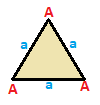
|
Isosceles { }∨( ) 
|
Scalene ( )∨( )∨( ) 
|
|---|---|---|
| (v:3; e:3) | (v:2+1; e:2+1) | (v:1+1+1; e:1+1+1) |
  | A | a
--+---+---
A | 3 | 2
--+---+---
a | 2 | 3
|
  | A B | a b
--+-----+-----
A | 2 * | 1 1
B | * 1 | 2 0
--+-----+-----
a | 1 1 | 2 *
b | 2 0 | * 1
|
| A B C | a b c --+-------+------- A | 1 * * | 0 1 1 B | * 1 * | 1 0 1 C | * * 1 | 1 1 0 --+-------+------- a | 0 1 1 | 1 * * b | 1 0 1 | * 1 * c | 1 1 0 | * * 1 |
Quadrilaterals edit

Quadrilaterals can be classified by symmetry, each with their own matrix. Quadrilaterals exist with dual pairs which will have the same matrix, rotated 180 degrees, with vertices and edges reversed. Squares and parallelograms, and general quadrilaterals are self-dual by class so their matrices are unchanged when rotated 180 degrees.
| Square {4} 
|
Rectangle { }×{ } 
|
Rhombus { }+{ } 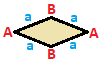
|
Parallelogram
|
|---|---|---|---|
| (v:4; e:4) | (v:4; e:2+2) | (v:2+2; e:4) | (v:2+2; e:2+2) |
  | A | a
--+---+---
A | 4 | 2
--+---+---
a | 2 | 4
|
  | A | a b
--+---+-----
A | 4 | 1 1
--+---+-----
a | 2 | 2 *
b | 2 | * 2
|
  | A B | a
--+-----+---
A | 2 * | 2
B | * 2 | 2
--+-----+---
a | 1 1 | 4
|
| A B | a b --+-----+----- A | 2 * | 1 1 B | * 2 | 1 1 --+-----+----- a | 1 1 | 2 * b | 1 1 | * 2 |
| Isosceles trapezoid { }||{ } 
|
Kite
|
General
| |
| (v:2+2; e:1+1+2) | (v:1+1+2; e:2+2) | (v:1+1+1+1; e:1+1+1+1) | |
  | A B | a b c
--+-----+-------
A | 2 * | 1 0 1
B | * 2 | 0 1 1
--+-----+------
a | 2 0 | 1 * *
b | 0 2 | * 1 *
c | 1 1 | * * 2
|
  | A B C | a b
--+-------+----
A | 1 * * | 2 0
B | * 1 * | 0 2
C | * * 2 | 1 1
--+-------+----
a | 1 0 1 | 2 *
b | 0 1 1 | * 2
|
| A B C D | a b c d --+---------+-------- A | 1 * * * | 1 0 0 1 B | * 1 * * | 1 1 0 0 C | * * 1 * | 0 1 1 0 D | * * * 1 | 0 0 1 1 --+---------+-------- a | 1 1 0 0 | 1 * * * b | 0 1 1 0 | * 1 * * c | 0 0 1 1 | * * 1 * d | 1 0 0 1 | * * * 1 | |
Complex polygons edit
The idea is also applicable for regular complex polygons, p{q}r constructed in :


The complex reflection group is p[q]r, order .[3][4]

Polyhedra edit
The idea can be applied in three dimensions by considering incidences of points, lines and planes, or j-spaces (0 ≤ j < 3), where each j-space is incident with Njk k-spaces (j ≠ k). Writing Nj for the number of j-spaces present, a given configuration may be represented by the matrix
- for Schläfli symbol {p,q}, with group order g = 4pq/(4 − (p − 2)(q − 2)).

Tetrahedron edit

Tetrahedra have matrices that can also be grouped by their symmetry, with a general tetrahedron having 14 rows and columns for the 4 vertices, 6 edges, and 4 faces. Tetrahedra are self-dual, and rotating the matices 180 degrees (swapping vertices and faces) will leave it unchanged.
| Regular (v:4; e:6; f:4) 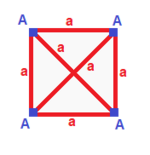
|
tetragonal disphenoid (v:4; e:2+4; f:4) 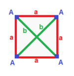
|
Rhombic disphenoid (v:4; e:2+2+2; f:4) 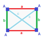
|
Digonal disphenoid (v:2+2; e:4+1+1; f:2+2) 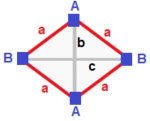
|
Phyllic disphenoid (v:2+2; e:2+2+1+1; f:2+2) 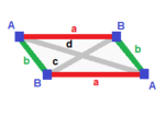
|
|---|---|---|---|---|
A| 4 | 3 | 3 ---+---+---+-- a| 2 | 6 | 2 ---+---+---+-- aaa| 3 | 3 | 4 |
A| 4 | 2 1 | 3 ---+---+-----+-- a| 2 | 4 * | 2 b| 2 | * 2 | 2 ---+---+-----+-- aab| 3 | 2 1 | 4 |
A| 4 | 1 1 1 | 3 ----+---+-------+-- a| 2 | 2 * * | 2 b| 2 | * 2 * | 2 c| 2 | * * 2 | 2 ----+---+-------+-- abc| 3 | 1 1 1 | 4 |
A| 2 * | 2 1 0 | 2 1 B| * 2 | 2 0 1 | 1 2 ---+-----+-------+---- a| 1 1 | 4 * * | 1 1 b| 2 0 | * 1 * | 2 0 c| 0 2 | * * 1 | 0 2 ---+-----+-------+---- aab| 2 1 | 2 1 0 | 2 * aac| 1 2 | 2 0 1 | * 2 |
A| 2 * | 1 0 1 1 | 1 2 B| * 2 | 1 1 1 0 | 2 1 ---+-----+---------+---- a| 1 1 | 2 * * * | 1 1 b| 1 1 | * 2 * * | 1 1 c| 0 2 | * * 1 * | 2 0 d| 2 0 | * * * 1 | 0 2 ---+-----+---------+---- abc| 1 2 | 1 1 1 0 | 2 * bcd| 2 1 | 1 1 0 1 | * 2 |
| Triangular pyramid (v:3+1; e:3+3; f:3+1) 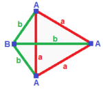
|
Mirrored spheroid (v:2+1+1; e:2+2+1+1; f:2+1+1) 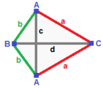
|
No symmetry (v:1+1+1+1; e:1+1+1+1+1+1; f:1+1+1+1) 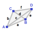
| ||
A| 3 * | 2 1 | 2 1 B| * 1 | 0 3 | 3 0 ---+-----+-----+---- a| 2 0 | 3 * | 1 1 b| 1 1 | * 3 | 2 0 ---+-----+-----+---- abb| 2 1 | 1 2 | 3 * aaa| 3 0 | 3 0 | * 1 |
A| 2 * * | 1 1 0 1 | 1 1 1 B| * 1 * | 2 0 1 0 | 0 2 1 C| * * 1 | 0 2 1 0 | 1 2 0 ---+-------+---------+------ a| 1 0 1 | 2 * * * | 0 1 1 b| 0 1 1 | * 2 * * | 1 1 0 c| 1 1 0 | * * 1 * | 0 2 0 d| 0 0 2 | * * * 1 | 1 0 1 ---+-------+---------+------ ABC| 1 1 1 | 1 1 1 0 | 2 * * ACC| 1 0 2 | 2 0 0 1 | * 1 * BCC| 0 1 2 | 0 2 0 1 | * * 1 |
A | 1 * * * | 1 1 1 0 0 0 | 1 1 1 0 B | * 1 * * | 1 0 0 1 1 0 | 1 1 0 1 C | * * 1 * | 0 1 0 1 0 1 | 1 0 1 1 D | * * * 1 | 0 0 1 0 1 1 | 0 1 1 1 ----+---------+-------------+-------- a | 1 1 0 0 | 1 * * * * * | 1 1 0 0 b | 1 0 1 0 | * 1 * * * * | 1 0 1 0 c | 1 0 0 1 | * * 1 * * * | 0 1 1 0 d | 0 1 1 0 | * * * 1 * * | 1 0 0 1 e | 0 1 0 1 | * * * * 1 * | 0 1 0 1 f | 0 0 1 1 | * * * * * 1 | 0 0 1 1 ----+---------+-------------+-------- ABC | 1 1 1 0 | 1 1 0 1 0 0 | 1 * * * ABD | 1 1 0 1 | 1 0 1 0 1 0 | * 1 * * ACD | 1 0 1 1 | 0 1 1 0 0 1 | * * 1 * BCD | 0 1 1 1 | 0 0 0 1 1 1 | * * * 1 | ||
Notes edit
References edit
- Coxeter, H.S.M. (1948), Regular Polytopes, Methuen and Co.
- Coxeter, H.S.M. (1991), Regular Complex Polytopes, Cambridge University Press, ISBN 0-521-39490-2
- Coxeter, H.S.M. (1999), "Self-dual configurations and regular graphs", The Beauty of Geometry, Dover, ISBN 0-486-40919-8