Covariant_formulation_of_classical_electromagnetism Knowpia

The covariant formulation of classical electromagnetism refers to ways of writing the laws of classical electromagnetism (in particular, Maxwell's equations and the Lorentz force) in a form that is manifestly invariant under Lorentz transformations, in the formalism of special relativity using rectilinear inertial coordinate systems. These expressions both make it simple to prove that the laws of classical electromagnetism take the same form in any inertial coordinate system, and also provide a way to translate the fields and forces from one frame to another. However, this is not as general as Maxwell's equations in curved spacetime or non-rectilinear coordinate systems.

This article uses the classical treatment of tensors and Einstein summation convention throughout and the Minkowski metric has the form $diag(+1, -1, -1, -1)$ . Where the equations are specified as holding in a vacuum, one could instead regard them as the formulation of Maxwell's equations in terms of total charge and current.

For a more general overview of the relationships between classical electromagnetism and special relativity, including various conceptual implications of this picture, see Classical electromagnetism and special relativity.

Covariant objectsEdit

Preliminary four-vectorsEdit

Lorentz tensors of the following kinds may be used in this article to describe bodies or particles:

four-displacement: $x^{\alpha }=(ct,\mathbf {x} )=(ct,x,y,z)\,.$
Four-velocity: $u^{\alpha }=\gamma (c,\mathbf {u} ),$ where γ(u) is the Lorentz factor at the 3-velocity u.
Four-momentum: $p^{\alpha }=(E/c,\mathbf {p} )=m_{0}u^{\alpha }$ where $\mathbf {p}$ is 3-momentum, $E$ is the total energy, and $m_{0}$ is rest mass.
Four-gradient: $\partial ^{\nu }={\frac {\partial }{\partial x_{\nu }}}=\left({\frac {1}{c}}{\frac {\partial }{\partial t}},-\mathbf {\nabla } \right)\,,$
The d'Alembertian operator is denoted ${\partial }^{2}$ , $\partial ^{2}={\frac {1}{c^{2}}}{\partial \over \partial t}{\partial \over \partial t}-\nabla ^{2}.$

The signs in the following tensor analysis depend on the convention used for the metric tensor. The convention used here is (+ − − −), corresponding to the Minkowski metric tensor:

\eta ^{\mu \nu }={\begin{pmatrix}1&0&0&0\\0&-1&0&0\\0&0&-1&0\\0&0&0&-1\end{pmatrix}}

Electromagnetic tensorEdit

The electromagnetic tensor is the combination of the electric and magnetic fields into a covariant antisymmetric tensor whose entries are B-field quantities.^[1]

F_{\alpha \beta }={\begin{pmatrix}0&E_{x}/c&E_{y}/c&E_{z}/c\\-E_{x}/c&0&-B_{z}&B_{y}\\-E_{y}/c&B_{z}&0&-B_{x}\\-E_{z}/c&-B_{y}&B_{x}&0\end{pmatrix}}

and the result of raising its indices is

F^{\mu \nu }\mathrel {\stackrel {\mathrm {def} }{=}} \eta ^{\mu \alpha }\,F_{\alpha \beta }\,\eta ^{\beta \nu }={\begin{pmatrix}0&-E_{x}/c&-E_{y}/c&-E_{z}/c\\E_{x}/c&0&-B_{z}&B_{y}\\E_{y}/c&B_{z}&0&-B_{x}\\E_{z}/c&-B_{y}&B_{x}&0\end{pmatrix}}\,.

where E is the electric field, B the magnetic field, and c the speed of light.

Four-currentEdit

The four-current is the contravariant four-vector which combines electric charge density ρ and electric current density j:

J^{\alpha }=(c\rho ,\mathbf {j} )\,.

Four-potentialEdit

The electromagnetic four-potential is a covariant four-vector containing the electric potential (also called the scalar potential) ϕ and magnetic vector potential (or vector potential) A, as follows:

A^{\alpha }=\left(\phi /c,\mathbf {A} \right)\,.

The differential of the electromagnetic potential is

F_{\alpha \beta }=\partial _{\alpha }A_{\beta }-\partial _{\beta }A_{\alpha }\,.

In the language of differential forms, which provides the generalisation to curved spacetimes, these are the components of a 1-form $A=A_{\alpha }dx^{\alpha }$ and a 2-form ${\textstyle F=dA={\frac {1}{2}}F_{\alpha \beta }dx^{\alpha }\wedge dx^{\beta }}$ respectively. Here, $d$ is the exterior derivative and $\wedge$ the wedge product.

Electromagnetic stress–energy tensorEdit

The electromagnetic stress–energy tensor can be interpreted as the flux density of the momentum four-vector, and is a contravariant symmetric tensor that is the contribution of the electromagnetic fields to the overall stress–energy tensor:

T^{\alpha \beta }={\begin{pmatrix}\varepsilon _{0}E^{2}/2+B^{2}/2\mu _{0}&S_{x}/c&S_{y}/c&S_{z}/c\\S_{x}/c&-\sigma _{xx}&-\sigma _{xy}&-\sigma _{xz}\\S_{y}/c&-\sigma _{yx}&-\sigma _{yy}&-\sigma _{yz}\\S_{z}/c&-\sigma _{zx}&-\sigma _{zy}&-\sigma _{zz}\end{pmatrix}}\,,

where $\varepsilon _{0}$ is the electric permittivity of vacuum, μ₀ is the magnetic permeability of vacuum, the Poynting vector is

\mathbf {S} ={\frac {1}{\mu _{0}}}\mathbf {E} \times \mathbf {B}

and the Maxwell stress tensor is given by

\sigma _{ij}=\varepsilon _{0}E_{i}E_{j}+{\frac {1}{\mu _{0}}}B_{i}B_{j}-\left({\frac {1}{2}}\varepsilon _{0}E^{2}+{\frac {1}{2\mu _{0}}}B^{2}\right)\delta _{ij}\,.

The electromagnetic field tensor F constructs the electromagnetic stress–energy tensor T by the equation:^[2]

T^{\alpha \beta }={\frac {1}{\mu _{0}}}\left(\eta ^{\alpha \nu }F_{\nu \gamma }F^{\gamma \beta }+{\frac {1}{4}}\eta ^{\alpha \beta }F_{\gamma \nu }F^{\gamma \nu }\right)

where η is the Minkowski metric tensor (with signature (+ − − −)). Notice that we use the fact that

\varepsilon _{0}\mu _{0}c^{2}=1\,,

which is predicted by Maxwell's equations.

Maxwell's equations in vacuumEdit

In vacuum (or for the microscopic equations, not including macroscopic material descriptions), Maxwell's equations can be written as two tensor equations.

The two inhomogeneous Maxwell's equations, Gauss's Law and Ampère's law (with Maxwell's correction) combine into (with (+ − − −) metric):^[3]

Gauss–Ampère law

$\partial _{\alpha }F^{\alpha \beta }=\mu _{0}J^{\beta }$

while the homogeneous equations – Faraday's law of induction and Gauss's law for magnetism combine to form $\partial ^{\sigma }F^{\mu \nu }+\partial ^{\mu }F^{\nu \sigma }+\partial ^{\nu }F^{\sigma \mu }=0$ , which may be written using Levi-Civita duality as:

Gauss–Faraday law

$\partial _{\alpha }\left({\tfrac {1}{2}}\varepsilon ^{\alpha \beta \gamma \delta }F_{\gamma \delta }\right)=0$

where F^αβ is the electromagnetic tensor, J^α is the four-current, ε^αβγδ is the Levi-Civita symbol, and the indices behave according to the Einstein summation convention.

Each of these tensor equations corresponds to four scalar equations, one for each value of β.

Using the antisymmetric tensor notation and comma notation for the partial derivative (see Ricci calculus), the second equation can also be written more compactly as:

F_{[\alpha \beta ,\gamma ]}=0.

In the absence of sources, Maxwell's equations reduce to:

\partial ^{\nu }\partial _{\nu }F^{\alpha \beta }\mathrel {\stackrel {\text{def}}{=}} \partial ^{2}F^{\alpha \beta }\mathrel {\stackrel {\text{def}}{=}} {1 \over c^{2}}{\partial ^{2}F^{\alpha \beta } \over {\partial t}^{2}}-\nabla ^{2}F^{\alpha \beta }=0\,,

which is an electromagnetic wave equation in the field strength tensor.

Maxwell's equations in the Lorenz gaugeEdit

The Lorenz gauge condition is a Lorentz-invariant gauge condition. (This can be contrasted with other gauge conditions such as the Coulomb gauge, which if it holds in one inertial frame will generally not hold in any other.) It is expressed in terms of the four-potential as follows:

\partial _{\alpha }A^{\alpha }=\partial ^{\alpha }A_{\alpha }=0\,.

In the Lorenz gauge, the microscopic Maxwell's equations can be written as:

{\partial }^{2}A^{\sigma }=\mu _{0}\,J^{\sigma }\,.

Lorentz forceEdit

Charged particleEdit

Lorentz force f on a charged particle (of charge q) in motion (instantaneous velocity v). The E field and B field vary in space and time.

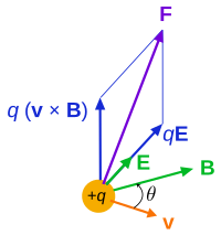
Electromagnetic (EM) fields affect the motion of electrically charged matter: due to the Lorentz force. In this way, EM fields can be detected (with applications in particle physics, and natural occurrences such as in aurorae). In relativistic form, the Lorentz force uses the field strength tensor as follows.^[4]

Expressed in terms of coordinate time t, it is:

{dp_{\alpha } \over {dt}}=q\,F_{\alpha \beta }\,{\frac {dx^{\beta }}{dt}},

where p_α is the four-momentum, q is the charge, and x^β is the position.

Expressed in frame-independent form, we have the four-force

{\frac {dp_{\alpha }}{d\tau }}\,=q\,F_{\alpha \beta }\,u^{\beta },

where u^β is the four-velocity, and τ is the particle's proper time, which is related to coordinate time by dt = γdτ.

Charge continuumEdit

Lorentz force per spatial volume f on a continuous charge distribution (charge density ρ) in motion.

The density of force due to electromagnetism, whose spatial part is the Lorentz force, is given by

f_{\alpha }=F_{\alpha \beta }J^{\beta }.

and is related to the electromagnetic stress–energy tensor by

f^{\alpha }=-{T^{\alpha \beta }}_{,\beta }\equiv -{\frac {\partial T^{\alpha \beta }}{\partial x^{\beta }}}.

Conservation lawsEdit

Electric chargeEdit

The continuity equation:

{J^{\beta }}_{,\beta }\mathrel {\overset {\text{def}}{\mathop {=} }} \partial _{\beta }J^{\beta }=\partial _{\beta }\partial _{\alpha }F^{\alpha \beta }/\mu _{0}=0.

expresses charge conservation.

Electromagnetic energy–momentumEdit

Using the Maxwell equations, one can see that the electromagnetic stress–energy tensor (defined above) satisfies the following differential equation, relating it to the electromagnetic tensor and the current four-vector

{T^{\alpha \beta }}_{,\beta }+F^{\alpha \beta }J_{\beta }=0

or

\eta _{\alpha \nu }{T^{\nu \beta }}_{,\beta }+F_{\alpha \beta }J^{\beta }=0,

which expresses the conservation of linear momentum and energy by electromagnetic interactions.

Covariant objects in matterEdit

Free and bound four-currentsEdit

In order to solve the equations of electromagnetism given here, it is necessary to add information about how to calculate the electric current, J^ν Frequently, it is convenient to separate the current into two parts, the free current and the bound current, which are modeled by different equations;

J^{\nu }={J^{\nu }}_{\text{free}}+{J^{\nu }}_{\text{bound}}\,,

where

{\begin{aligned}{J^{\nu }}_{\text{free}}={\begin{pmatrix}c\rho _{\text{free}},&\mathbf {J} _{\text{free}}\end{pmatrix}}&={\begin{pmatrix}c\nabla \cdot \mathbf {D} ,&-{\frac {\partial \mathbf {D} }{\partial t}}+\nabla \times \mathbf {H} \end{pmatrix}}\,,\\{J^{\nu }}_{\text{bound}}={\begin{pmatrix}c\rho _{\text{bound}},&\mathbf {J} _{\text{bound}}\end{pmatrix}}&={\begin{pmatrix}-c\nabla \cdot \mathbf {P} ,&{\frac {\partial \mathbf {P} }{\partial t}}+\nabla \times \mathbf {M} \end{pmatrix}}\,.\end{aligned}}

Maxwell's macroscopic equations have been used, in addition the definitions of the electric displacement D and the magnetic intensity H:

{\begin{aligned}\mathbf {D} &=\varepsilon _{0}\mathbf {E} +\mathbf {P} ,\\\mathbf {H} &={\frac {1}{\mu _{0}}}\mathbf {B} -\mathbf {M} \,.\end{aligned}}

where M is the magnetization and P the electric polarization.

Magnetization–polarization tensorEdit

The bound current is derived from the P and M fields which form an antisymmetric contravariant magnetization-polarization tensor ^[1]

{\mathcal {M}}^{\mu \nu }={\begin{pmatrix}0&P_{x}c&P_{y}c&P_{z}c\\-P_{x}c&0&-M_{z}&M_{y}\\-P_{y}c&M_{z}&0&-M_{x}\\-P_{z}c&-M_{y}&M_{x}&0\end{pmatrix}},

which determines the bound current

{J^{\nu }}_{\text{bound}}=\partial _{\mu }{\mathcal {M}}^{\mu \nu }\,.

Electric displacement tensorEdit

If this is combined with F^μν we get the antisymmetric contravariant electromagnetic displacement tensor which combines the D and H fields as follows:

{\mathcal {D}}^{\mu \nu }={\begin{pmatrix}0&-D_{x}c&-D_{y}c&-D_{z}c\\D_{x}c&0&-H_{z}&H_{y}\\D_{y}c&H_{z}&0&-H_{x}\\D_{z}c&-H_{y}&H_{x}&0\end{pmatrix}}.

The three field tensors are related by:

{\mathcal {D}}^{\mu \nu }={\frac {1}{\mu _{0}}}F^{\mu \nu }-{\mathcal {M}}^{\mu \nu }

which is equivalent to the definitions of the D and H fields given above.

Maxwell's equations in matterEdit

The result is that Ampère's law,

\mathbf {\nabla } \times \mathbf {H} =\mathbf {J} _{\text{free}}+{\frac {\partial \mathbf {D} }{\partial t}},

and Gauss's law,

\mathbf {\nabla } \cdot \mathbf {D} =\rho _{\text{free}},

combine into one equation:

Gauss–Ampère law (matter)

${J^{\nu }}_{\text{free}}=\partial _{\mu }{\mathcal {D}}^{\mu \nu }$

The bound current and free current as defined above are automatically and separately conserved

{\begin{aligned}\partial _{\nu }{J^{\nu }}_{\text{bound}}&=0\,\\\partial _{\nu }{J^{\nu }}_{\text{free}}&=0\,.\end{aligned}}

Constitutive equationsEdit

VacuumEdit

In vacuum, the constitutive relations between the field tensor and displacement tensor are:

\mu _{0}{\mathcal {D}}^{\mu \nu }=\eta ^{\mu \alpha }F_{\alpha \beta }\eta ^{\beta \nu }\,.

Antisymmetry reduces these 16 equations to just six independent equations. Because it is usual to define F^μν by

F^{\mu \nu }=\eta ^{\mu \alpha }F_{\alpha \beta }\eta ^{\beta \nu },

the constitutive equations may, in vacuum, be combined with the Gauss–Ampère law to get:

\partial _{\beta }F^{\alpha \beta }=\mu _{0}J^{\alpha }.

The electromagnetic stress–energy tensor in terms of the displacement is:

T_{\alpha }{}^{\pi }=F_{\alpha \beta }{\mathcal {D}}^{\pi \beta }-{\frac {1}{4}}\delta _{\alpha }^{\pi }F_{\mu \nu }{\mathcal {D}}^{\mu \nu },

where δ_α^π is the Kronecker delta. When the upper index is lowered with η, it becomes symmetric and is part of the source of the gravitational field.

Linear, nondispersive matterEdit

Thus we have reduced the problem of modeling the current, J^ν to two (hopefully) easier problems — modeling the free current, J^ν_free and modeling the magnetization and polarization, ${\mathcal {M}}^{\mu \nu }$ . For example, in the simplest materials at low frequencies, one has

{\begin{aligned}\mathbf {J} _{\text{free}}&=\sigma \mathbf {E} \,\\\mathbf {P} &=\varepsilon _{0}\chi _{e}\mathbf {E} \,\\\mathbf {M} &=\chi _{m}\mathbf {H} \,\end{aligned}}

where one is in the instantaneously comoving inertial frame of the material, σ is its electrical conductivity, χ_e is its electric susceptibility, and χ_m is its magnetic susceptibility.

The constitutive relations between the ${\mathcal {D}}$ and F tensors, proposed by Minkowski for a linear materials (that is, E is proportional to D and B proportional to H), are:

{\begin{aligned}{\mathcal {D}}^{\mu \nu }u_{\nu }&=c^{2}\varepsilon F^{\mu \nu }u_{\nu }\\{\star {\mathcal {D}}^{\mu \nu }}u_{\nu }&={\frac {1}{\mu }}{\star F^{\mu \nu }}u_{\nu }\end{aligned}}

where u is the four-velocity of material, ε and μ are respectively the proper permittivity and permeability of the material (i.e. in rest frame of material), $\star$ and denotes the Hodge star operator.

Lagrangian for classical electrodynamicsEdit

VacuumEdit

The Lagrangian density for classical electrodynamics is composed by two components: a field component and a source component:

{\mathcal {L}}\,=\,{\mathcal {L}}_{\text{field}}+{\mathcal {L}}_{\text{int}}=-{\frac {1}{4\mu _{0}}}F^{\alpha \beta }F_{\alpha \beta }-A_{\alpha }J^{\alpha }\,.

In the interaction term, the four-current should be understood as an abbreviation of many terms expressing the electric currents of other charged fields in terms of their variables; the four-current is not itself a fundamental field.

The Lagrange equations for the electromagnetic lagrangian density ${\mathcal {L}}{\mathord {\left(A_{\alpha },\partial _{\beta }A_{\alpha }\right)}}$ can be stated as follows:

\partial _{\beta }\left[{\frac {\partial {\mathcal {L}}}{\partial (\partial _{\beta }A_{\alpha })}}\right]-{\frac {\partial {\mathcal {L}}}{\partial A_{\alpha }}}=0\,.

Noting

{\begin{aligned}F^{\lambda \sigma }&=F_{\mu \nu }\eta ^{\mu \lambda }\eta ^{\nu \sigma },\\F_{\mu \nu }&=\partial _{\mu }A_{\nu }-\partial _{\nu }A_{\mu }\,\\{\partial \left(\partial _{\mu }A_{\nu }\right) \over \partial \left(\partial _{\rho }A_{\sigma }\right)}&=\delta _{\mu }^{\rho }\delta _{\nu }^{\sigma }\end{aligned}}

the expression inside the square bracket is

{\begin{aligned}{\frac {\partial {\mathcal {L}}}{\partial (\partial _{\beta }A_{\alpha })}}&=-\ {\frac {1}{4\mu _{0}}}\ {\frac {\partial \left(F_{\mu \nu }\eta ^{\mu \lambda }\eta ^{\nu \sigma }F_{\lambda \sigma }\right)}{\partial \left(\partial _{\beta }A_{\alpha }\right)}}\\&=-\ {\frac {1}{4\mu _{0}}}\ \eta ^{\mu \lambda }\eta ^{\nu \sigma }\left(F_{\lambda \sigma }\left(\delta _{\mu }^{\beta }\delta _{\nu }^{\alpha }-\delta _{\nu }^{\beta }\delta _{\mu }^{\alpha }\right)+F_{\mu \nu }\left(\delta _{\lambda }^{\beta }\delta _{\sigma }^{\alpha }-\delta _{\sigma }^{\beta }\delta _{\lambda }^{\alpha }\right)\right)\\&=-\ {\frac {F^{\beta \alpha }}{\mu _{0}}}\,.\end{aligned}}

The second term is

{\frac {\partial {\mathcal {L}}}{\partial A_{\alpha }}}=-J^{\alpha }\,.

Therefore, the electromagnetic field's equations of motion are

{\frac {\partial F^{\beta \alpha }}{\partial x^{\beta }}}=\mu _{0}J^{\alpha }\,.

which is the Gauss–Ampère equation above.

MatterEdit

Separating the free currents from the bound currents, another way to write the Lagrangian density is as follows:

{\mathcal {L}}\,=\,-{\frac {1}{4\mu _{0}}}F^{\alpha \beta }F_{\alpha \beta }-A_{\alpha }J_{\text{free}}^{\alpha }+{\frac {1}{2}}F_{\alpha \beta }{\mathcal {M}}^{\alpha \beta }\,.

Using Lagrange equation, the equations of motion for ${\mathcal {D}}^{\mu \nu }$ can be derived.

The equivalent expression in vector notation is:

{\mathcal {L}}\,=\,{\frac {1}{2}}\left(\varepsilon _{0}E^{2}-{\frac {1}{\mu _{0}}}B^{2}\right)-\phi \,\rho _{\text{free}}+\mathbf {A} \cdot \mathbf {J} _{\text{free}}+\mathbf {E} \cdot \mathbf {P} +\mathbf {B} \cdot \mathbf {M} \,.

Notes and referencesEdit

^ ^a ^b Vanderlinde, Jack (2004), classical electromagnetic theory, Springer, pp. 313–328, ISBN 9781402026997
^ Classical Electrodynamics, Jackson, 3rd edition, page 609
^ Classical Electrodynamics by Jackson, 3rd Edition, Chapter 11 Special Theory of Relativity
^ The assumption is made that no forces other than those originating in E and B are present, that is, no gravitational, weak or strong forces.