


Summary
In physics, equations of motion are equations that describe the behavior of a physical system in terms of its motion as a function of time.[1] More specifically, the equations of motion describe the behavior of a physical system as a set of mathematical functions in terms of dynamic variables. These variables are usually spatial coordinates and time, but may include momentum components. The most general choice are generalized coordinates which can be any convenient variables characteristic of the physical system.[2] The functions are defined in a Euclidean space in classical mechanics, but are replaced by curved spaces in relativity. If the dynamics of a system is known, the equations are the solutions for the differential equations describing the motion of the dynamics.


Types edit
There are two main descriptions of motion: dynamics and kinematics. Dynamics is general, since the momenta, forces and energy of the particles are taken into account. In this instance, sometimes the term dynamics refers to the differential equations that the system satisfies (e.g., Newton's second law or Euler–Lagrange equations), and sometimes to the solutions to those equations.
However, kinematics is simpler. It concerns only variables derived from the positions of objects and time. In circumstances of constant acceleration, these simpler equations of motion are usually referred to as the SUVAT equations, arising from the definitions of kinematic quantities: displacement (s), initial velocity (u), final velocity (v), acceleration (a), and time (t).
A differential equation of motion, usually identified as some physical law (for example, F = ma) and applying definitions of physical quantities, is used to set up an equation for the problem.[clarification needed] Solving the differential equation will lead to a general solution with arbitrary constants, the arbitrariness corresponding to a family of solutions. A particular solution can be obtained by setting the initial values, which fixes the values of the constants.
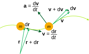
To state this formally, in general an equation of motion M is a function of the position r of the object, its velocity (the first time derivative of r, v = dr/dt), and its acceleration (the second derivative of r, a = d2r/dt2), and time t. Euclidean vectors in 3D are denoted throughout in bold. This is equivalent to saying an equation of motion in r is a second-order ordinary differential equation (ODE) in r,
![{\displaystyle M\left[\mathbf {r} (t),\mathbf {\dot {r}} (t),\mathbf {\ddot {r}} (t),t\right]=0\,,}](https://wikimedia.org/api/rest_v1/media/math/render/svg/969c32e88d55826a347715bee49544f4ab6bf67a)
where t is time, and each overdot denotes one time derivative. The initial conditions are given by the constant values at t = 0,

The solution r(t) to the equation of motion, with specified initial values, describes the system for all times t after t = 0. Other dynamical variables like the momentum p of the object, or quantities derived from r and p like angular momentum, can be used in place of r as the quantity to solve for from some equation of motion, although the position of the object at time t is by far the most sought-after quantity.
Sometimes, the equation will be linear and is more likely to be exactly solvable. In general, the equation will be non-linear, and cannot be solved exactly so a variety of approximations must be used. The solutions to nonlinear equations may show chaotic behavior depending on how sensitive the system is to the initial conditions.
History edit
Kinematics, dynamics and the mathematical models of the universe developed incrementally over three millennia, thanks to many thinkers, only some of whose names we know. In antiquity, priests, astrologers and astronomers predicted solar and lunar eclipses, the solstices and the equinoxes of the Sun and the period of the Moon. But they had nothing other than a set of algorithms to guide them. Equations of motion were not written down for another thousand years.
Medieval scholars in the thirteenth century — for example at the relatively new universities in Oxford and Paris — drew on ancient mathematicians (Euclid and Archimedes) and philosophers (Aristotle) to develop a new body of knowledge, now called physics.
At Oxford, Merton College sheltered a group of scholars devoted to natural science, mainly physics, astronomy and mathematics, who were of similar stature to the intellectuals at the University of Paris. Thomas Bradwardine extended Aristotelian quantities such as distance and velocity, and assigned intensity and extension to them. Bradwardine suggested an exponential law involving force, resistance, distance, velocity and time. Nicholas Oresme further extended Bradwardine's arguments. The Merton school proved that the quantity of motion of a body undergoing a uniformly accelerated motion is equal to the quantity of a uniform motion at the speed achieved halfway through the accelerated motion.
For writers on kinematics before Galileo, since small time intervals could not be measured, the affinity between time and motion was obscure. They used time as a function of distance, and in free fall, greater velocity as a result of greater elevation. Only Domingo de Soto, a Spanish theologian, in his commentary on Aristotle's Physics published in 1545, after defining "uniform difform" motion (which is uniformly accelerated motion) – the word velocity was not used – as proportional to time, declared correctly that this kind of motion was identifiable with freely falling bodies and projectiles, without his proving these propositions or suggesting a formula relating time, velocity and distance. De Soto's comments are remarkably correct regarding the definitions of acceleration (acceleration was a rate of change of motion (velocity) in time) and the observation that acceleration would be negative during ascent.
Discourses such as these spread throughout Europe, shaping the work of Galileo Galilei and others, and helped in laying the foundation of kinematics.[3] Galileo deduced the equation s = 1/2gt2 in his work geometrically,[4] using the Merton rule, now known as a special case of one of the equations of kinematics.
Galileo was the first to show that the path of a projectile is a parabola. Galileo had an understanding of centrifugal force and gave a correct definition of momentum. This emphasis of momentum as a fundamental quantity in dynamics is of prime importance. He measured momentum by the product of velocity and weight; mass is a later concept, developed by Huygens and Newton. In the swinging of a simple pendulum, Galileo says in Discourses[5] that "every momentum acquired in the descent along an arc is equal to that which causes the same moving body to ascend through the same arc." His analysis on projectiles indicates that Galileo had grasped the first law and the second law of motion. He did not generalize and make them applicable to bodies not subject to the earth's gravitation. That step was Newton's contribution.
The term "inertia" was used by Kepler who applied it to bodies at rest. (The first law of motion is now often called the law of inertia.)
Galileo did not fully grasp the third law of motion, the law of the equality of action and reaction, though he corrected some errors of Aristotle. With Stevin and others Galileo also wrote on statics. He formulated the principle of the parallelogram of forces, but he did not fully recognize its scope.
Galileo also was interested by the laws of the pendulum, his first observations of which were as a young man. In 1583, while he was praying in the cathedral at Pisa, his attention was arrested by the motion of the great lamp lighted and left swinging, referencing his own pulse for time keeping. To him the period appeared the same, even after the motion had greatly diminished, discovering the isochronism of the pendulum.
More careful experiments carried out by him later, and described in his Discourses, revealed the period of oscillation varies with the square root of length but is independent of the mass the pendulum.
Thus we arrive at René Descartes, Isaac Newton, Gottfried Leibniz, et al.; and the evolved forms of the equations of motion that begin to be recognized as the modern ones.
Later the equations of motion also appeared in electrodynamics, when describing the motion of charged particles in electric and magnetic fields, the Lorentz force is the general equation which serves as the definition of what is meant by an electric field and magnetic field. With the advent of special relativity and general relativity, the theoretical modifications to spacetime meant the classical equations of motion were also modified to account for the finite speed of light, and curvature of spacetime. In all these cases the differential equations were in terms of a function describing the particle's trajectory in terms of space and time coordinates, as influenced by forces or energy transformations.[6]
However, the equations of quantum mechanics can also be considered "equations of motion", since they are differential equations of the wavefunction, which describes how a quantum state behaves analogously using the space and time coordinates of the particles. There are analogs of equations of motion in other areas of physics, for collections of physical phenomena that can be considered waves, fluids, or fields.
Kinematic equations for one particle edit
Kinematic quantities edit
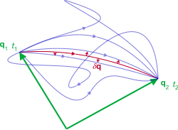
From the instantaneous position r = r(t), instantaneous meaning at an instant value of time t, the instantaneous velocity v = v(t) and acceleration a = a(t) have the general, coordinate-independent definitions;[7]

Notice that velocity always points in the direction of motion, in other words for a curved path it is the tangent vector. Loosely speaking, first order derivatives are related to tangents of curves. Still for curved paths, the acceleration is directed towards the center of curvature of the path. Again, loosely speaking, second order derivatives are related to curvature.
The rotational analogues are the "angular vector" (angle the particle rotates about some axis) θ = θ(t), angular velocity ω = ω(t), and angular acceleration α = α(t):

where n̂ is a unit vector in the direction of the axis of rotation, and θ is the angle the object turns through about the axis.
The following relation holds for a point-like particle, orbiting about some axis with angular velocity ω:[8]

where r is the position vector of the particle (radial from the rotation axis) and v the tangential velocity of the particle. For a rotating continuum rigid body, these relations hold for each point in the rigid body.
Uniform acceleration edit
The differential equation of motion for a particle of constant or uniform acceleration in a straight line is simple: the acceleration is constant, so the second derivative of the position of the object is constant. The results of this case are summarized below.
Constant translational acceleration in a straight line edit
These equations apply to a particle moving linearly, in three dimensions in a straight line with constant acceleration.[9] Since the position, velocity, and acceleration are collinear (parallel, and lie on the same line) – only the magnitudes of these vectors are necessary, and because the motion is along a straight line, the problem effectively reduces from three dimensions to one.
![{\displaystyle {\begin{aligned}v&=at+v_{0}&[1]\\r&=r_{0}+v_{0}t+{\tfrac {1}{2}}{a}t^{2}&[2]\\r&=r_{0}+{\tfrac {1}{2}}\left(v+v_{0}\right)t&[3]\\v^{2}&=v_{0}^{2}+2a\left(r-r_{0}\right)&[4]\\r&=r_{0}+vt-{\tfrac {1}{2}}{a}t^{2}&[5]\\\end{aligned}}}](https://wikimedia.org/api/rest_v1/media/math/render/svg/346e3b192498f7c6c4deca12702f8f427948fd30)
where:
- r0 is the particle's initial position
- r is the particle's final position
- v0 is the particle's initial velocity
- v is the particle's final velocity
- a is the particle's acceleration
- t is the time interval
Equations [1] and [2] are from integrating the definitions of velocity and acceleration,[9] subject to the initial conditions r(t0) = r0 and v(t0) = v0;
![{\displaystyle {\begin{aligned}\mathbf {v} &=\int \mathbf {a} dt=\mathbf {a} t+\mathbf {v} _{0}\,,&[1]\\\mathbf {r} &=\int (\mathbf {a} t+\mathbf {v} _{0})dt={\frac {\mathbf {a} t^{2}}{2}}+\mathbf {v} _{0}t+\mathbf {r} _{0}\,,&[2]\\\end{aligned}}}](https://wikimedia.org/api/rest_v1/media/math/render/svg/4621491fedc591b23d07a1f7896fcf12c5b4bdba)
in magnitudes,
![{\displaystyle {\begin{aligned}v&=at+v_{0}\,,&[1]\\r&={\frac {{a}t^{2}}{2}}+v_{0}t+r_{0}\,.&[2]\\\end{aligned}}}](https://wikimedia.org/api/rest_v1/media/math/render/svg/01077b6a5bf0449acaff5e05f0102fdd1f84e9b4)
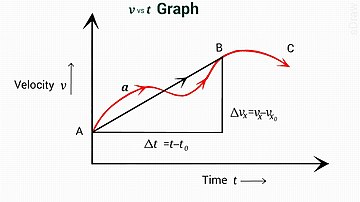
Equation [3] involves the average velocity v + v0/2. Intuitively, the velocity increases linearly, so the average velocity multiplied by time is the distance traveled while increasing the velocity from v0 to v, as can be illustrated graphically by plotting velocity against time as a straight line graph. Algebraically, it follows from solving [1] for

and substituting into [2]

then simplifying to get

or in magnitudes
![{\displaystyle r=r_{0}+\left({\frac {v+v_{0}}{2}}\right)t\quad [3]}](https://wikimedia.org/api/rest_v1/media/math/render/svg/3c8d0cd441e58cf8f118d4e89eaf8462a45fb02a)
From [3],

substituting for t in [1]:
![{\displaystyle {\begin{aligned}v&=a\left(r-r_{0}\right)\left({\frac {2}{v+v_{0}}}\right)+v_{0}\\v\left(v+v_{0}\right)&=2a\left(r-r_{0}\right)+v_{0}\left(v+v_{0}\right)\\v^{2}+vv_{0}&=2a\left(r-r_{0}\right)+v_{0}v+v_{0}^{2}\\v^{2}&=v_{0}^{2}+2a\left(r-r_{0}\right)&[4]\\\end{aligned}}}](https://wikimedia.org/api/rest_v1/media/math/render/svg/a7823eb6a835c32f8c6e780b7918ef7255c17b6d)
From [3],

substituting into [2]:
![{\displaystyle {\begin{aligned}r&={\frac {{a}t^{2}}{2}}+2r-2r_{0}-vt+r_{0}\\0&={\frac {{a}t^{2}}{2}}+r-r_{0}-vt\\r&=r_{0}+vt-{\frac {{a}t^{2}}{2}}&[5]\end{aligned}}}](https://wikimedia.org/api/rest_v1/media/math/render/svg/be5b09f6ca22b9d8cb5ca6ecd1cdd10d19ecb4f2)
Usually only the first 4 are needed, the fifth is optional.
Here a is constant acceleration, or in the case of bodies moving under the influence of gravity, the standard gravity g is used. Note that each of the equations contains four of the five variables, so in this situation it is sufficient to know three out of the five variables to calculate the remaining two.
In elementary physics the same formulae are frequently written in different notation as:
![{\displaystyle {\begin{aligned}v&=u+at&[1]\\s&=ut+{\tfrac {1}{2}}at^{2}&[2]\\s&={\tfrac {1}{2}}(u+v)t&[3]\\v^{2}&=u^{2}+2as&[4]\\s&=vt-{\tfrac {1}{2}}at^{2}&[5]\\\end{aligned}}}](https://wikimedia.org/api/rest_v1/media/math/render/svg/1246ab112ef8137bfed9cffd49530fa032bb9f09)
where u has replaced v0, s replaces r - r0. They are often referred to as the SUVAT equations, where "SUVAT" is an acronym from the variables: s = displacement, u = initial velocity, v = final velocity, a = acceleration, t = time.[10][11]
Constant linear acceleration in any direction edit

The initial position, initial velocity, and acceleration vectors need not be collinear, and the equations of motion take an almost identical form. The only difference is that the square magnitudes of the velocities require the dot product. The derivations are essentially the same as in the collinear case,
![{\displaystyle {\begin{aligned}\mathbf {v} &=\mathbf {a} t+\mathbf {v} _{0}&[1]\\\mathbf {r} &=\mathbf {r} _{0}+\mathbf {v} _{0}t+{\tfrac {1}{2}}\mathbf {a} t^{2}&[2]\\\mathbf {r} &=\mathbf {r} _{0}+{\tfrac {1}{2}}\left(\mathbf {v} +\mathbf {v} _{0}\right)t&[3]\\\mathbf {v} ^{2}&=\mathbf {v} _{0}^{2}+2\mathbf {a} \cdot \left(\mathbf {r} -\mathbf {r} _{0}\right)&[4]\\\mathbf {r} &=\mathbf {r} _{0}+\mathbf {v} t-{\tfrac {1}{2}}\mathbf {a} t^{2}&[5]\\\end{aligned}}}](https://wikimedia.org/api/rest_v1/media/math/render/svg/c757b958c1607b01cc40d06258309a93783ace8f)


Applications edit
Elementary and frequent examples in kinematics involve projectiles, for example a ball thrown upwards into the air. Given initial velocity u, one can calculate how high the ball will travel before it begins to fall. The acceleration is local acceleration of gravity g. While these quantities appear to be scalars, the direction of displacement, speed and acceleration is important. They could in fact be considered as unidirectional vectors. Choosing s to measure up from the ground, the acceleration a must be in fact −g, since the force of gravity acts downwards and therefore also the acceleration on the ball due to it.
At the highest point, the ball will be at rest: therefore v = 0. Using equation [4] in the set above, we have:

Substituting and cancelling minus signs gives:

Constant circular acceleration edit
The analogues of the above equations can be written for rotation. Again these axial vectors must all be parallel to the axis of rotation, so only the magnitudes of the vectors are necessary,

where α is the constant angular acceleration, ω is the angular velocity, ω0 is the initial angular velocity, θ is the angle turned through (angular displacement), θ0 is the initial angle, and t is the time taken to rotate from the initial state to the final state.
General planar motion edit

These are the kinematic equations for a particle traversing a path in a plane, described by position r = r(t).[12] They are simply the time derivatives of the position vector in plane polar coordinates using the definitions of physical quantities above for angular velocity ω and angular acceleration α. These are instantaneous quantities which change with time.
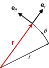
The position of the particle is

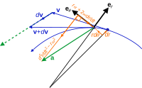
where êr and êθ are the polar unit vectors. Differentiating with respect to time gives the velocity

with radial component dr/dt and an additional component rω due to the rotation. Differentiating with respect to time again obtains the acceleration

which breaks into the radial acceleration d2r/dt2, centripetal acceleration –rω2, Coriolis acceleration 2ωdr/dt, and angular acceleration rα.
Special cases of motion described by these equations are summarized qualitatively in the table below. Two have already been discussed above, in the cases that either the radial components or the angular components are zero, and the non-zero component of motion describes uniform acceleration.
| State of motion | Constant r | r linear in t | r quadratic in t | r non-linear in t |
|---|---|---|---|---|
| Constant θ | Stationary | Uniform translation (constant translational velocity) | Uniform translational acceleration | Non-uniform translation |
| θ linear in t | Uniform angular motion in a circle (constant angular velocity) | Uniform angular motion in a spiral, constant radial velocity | Angular motion in a spiral, constant radial acceleration | Angular motion in a spiral, varying radial acceleration |
| θ quadratic in t | Uniform angular acceleration in a circle | Uniform angular acceleration in a spiral, constant radial velocity | Uniform angular acceleration in a spiral, constant radial acceleration | Uniform angular acceleration in a spiral, varying radial acceleration |
| θ non-linear in t | Non-uniform angular acceleration in a circle | Non-uniform angular acceleration in a spiral, constant radial velocity | Non-uniform angular acceleration in a spiral, constant radial acceleration | Non-uniform angular acceleration in a spiral, varying radial acceleration |
General 3D motions edit
In 3D space, the equations in spherical coordinates (r, θ, φ) with corresponding unit vectors êr, êθ and êφ, the position, velocity, and acceleration generalize respectively to

In the case of a constant φ this reduces to the planar equations above.
Dynamic equations of motion edit
Newtonian mechanics edit
The first general equation of motion developed was Newton's second law of motion. In its most general form it states the rate of change of momentum p = p(t) = mv(t) of an object equals the force F = F(x(t), v(t), t) acting on it,[13]: 1112

The force in the equation is not the force the object exerts. Replacing momentum by mass times velocity, the law is also written more famously as

since m is a constant in Newtonian mechanics.
Newton's second law applies to point-like particles, and to all points in a rigid body. They also apply to each point in a mass continuum, like deformable solids or fluids, but the motion of the system must be accounted for; see material derivative. In the case the mass is not constant, it is not sufficient to use the product rule for the time derivative on the mass and velocity, and Newton's second law requires some modification consistent with conservation of momentum; see variable-mass system.
It may be simple to write down the equations of motion in vector form using Newton's laws of motion, but the components may vary in complicated ways with spatial coordinates and time, and solving them is not easy. Often there is an excess of variables to solve for the problem completely, so Newton's laws are not always the most efficient way to determine the motion of a system. In simple cases of rectangular geometry, Newton's laws work fine in Cartesian coordinates, but in other coordinate systems can become dramatically complex.
The momentum form is preferable since this is readily generalized to more complex systems, such as special and general relativity (see four-momentum).[13]: 112 It can also be used with the momentum conservation. However, Newton's laws are not more fundamental than momentum conservation, because Newton's laws are merely consistent with the fact that zero resultant force acting on an object implies constant momentum, while a resultant force implies the momentum is not constant. Momentum conservation is always true for an isolated system not subject to resultant forces.
For a number of particles (see many body problem), the equation of motion for one particle i influenced by other particles is[7][1]

where pi is the momentum of particle i, Fij is the force on particle i by particle j, and FE is the resultant external force due to any agent not part of system. Particle i does not exert a force on itself.
Euler's laws of motion are similar to Newton's laws, but they are applied specifically to the motion of rigid bodies. The Newton–Euler equations combine the forces and torques acting on a rigid body into a single equation.
Newton's second law for rotation takes a similar form to the translational case,[13]

by equating the torque acting on the body to the rate of change of its angular momentum L. Analogous to mass times acceleration, the moment of inertia tensor I depends on the distribution of mass about the axis of rotation, and the angular acceleration is the rate of change of angular velocity,

Again, these equations apply to point like particles, or at each point of a rigid body.
Likewise, for a number of particles, the equation of motion for one particle i is[7]

where Li is the angular momentum of particle i, τij the torque on particle i by particle j, and τE is resultant external torque (due to any agent not part of system). Particle i does not exert a torque on itself.
Applications edit
Some examples[14] of Newton's law include describing the motion of a simple pendulum,

and a damped, sinusoidally driven harmonic oscillator,

For describing the motion of masses due to gravity, Newton's law of gravity can be combined with Newton's second law. For two examples, a ball of mass m thrown in the air, in air currents (such as wind) described by a vector field of resistive forces R = R(r, t),

where G is the gravitational constant, M the mass of the Earth, and A = R/m is the acceleration of the projectile due to the air currents at position r and time t.
The classical N-body problem for N particles each interacting with each other due to gravity is a set of N nonlinear coupled second order ODEs,

where i = 1, 2, ..., N labels the quantities (mass, position, etc.) associated with each particle.
Analytical mechanics edit
Using all three coordinates of 3D space is unnecessary if there are constraints on the system. If the system has N degrees of freedom, then one can use a set of N generalized coordinates q(t) = [q1(t), q2(t) ... qN(t)], to define the configuration of the system. They can be in the form of arc lengths or angles. They are a considerable simplification to describe motion, since they take advantage of the intrinsic constraints that limit the system's motion, and the number of coordinates is reduced to a minimum. The time derivatives of the generalized coordinates are the generalized velocities

The Euler–Lagrange equations are[2][16]

where the Lagrangian is a function of the configuration q and its time rate of change dq/dt (and possibly time t)
![{\displaystyle L=L\left[\mathbf {q} (t),\mathbf {\dot {q}} (t),t\right]\,.}](https://wikimedia.org/api/rest_v1/media/math/render/svg/9a30f80cbaa05dc7438902e9efb67fbad8ea096c)
Setting up the Lagrangian of the system, then substituting into the equations and evaluating the partial derivatives and simplifying, a set of coupled N second order ODEs in the coordinates are obtained.
Hamilton's equations are[2][16]

where the Hamiltonian
![{\displaystyle H=H\left[\mathbf {q} (t),\mathbf {p} (t),t\right]\,,}](https://wikimedia.org/api/rest_v1/media/math/render/svg/aecc975922b815e9bb266e1e3158865400b860c7)
is a function of the configuration q and conjugate "generalized" momenta

in which ∂/∂q = (∂/∂q1, ∂/∂q2, …, ∂/∂qN) is a shorthand notation for a vector of partial derivatives with respect to the indicated variables (see for example matrix calculus for this denominator notation), and possibly time t,
Setting up the Hamiltonian of the system, then substituting into the equations and evaluating the partial derivatives and simplifying, a set of coupled 2N first order ODEs in the coordinates qi and momenta pi are obtained.
The Hamilton–Jacobi equation is[2]

where
![{\displaystyle S[\mathbf {q} ,t]=\int _{t_{1}}^{t_{2}}L(\mathbf {q} ,\mathbf {\dot {q}} ,t)\,dt\,,}](https://wikimedia.org/api/rest_v1/media/math/render/svg/0dde602b4562727a396922b4b680ebe4afdc9828)
is Hamilton's principal function, also called the classical action is a functional of L. In this case, the momenta are given by

Although the equation has a simple general form, for a given Hamiltonian it is actually a single first order non-linear PDE, in N + 1 variables. The action S allows identification of conserved quantities for mechanical systems, even when the mechanical problem itself cannot be solved fully, because any differentiable symmetry of the action of a physical system has a corresponding conservation law, a theorem due to Emmy Noether.
All classical equations of motion can be derived from the variational principle known as Hamilton's principle of least action

stating the path the system takes through the configuration space is the one with the least action S.
Electrodynamics edit
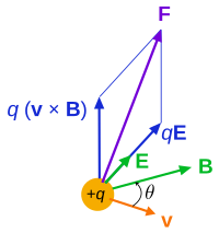
In electrodynamics, the force on a charged particle of charge q is the Lorentz force:[17]

Combining with Newton's second law gives a first order differential equation of motion, in terms of position of the particle:

or its momentum:

The same equation can be obtained using the Lagrangian (and applying Lagrange's equations above) for a charged particle of mass m and charge q:[16]

where A and ϕ are the electromagnetic scalar and vector potential fields. The Lagrangian indicates an additional detail: the canonical momentum in Lagrangian mechanics is given by:

Alternatively the Hamiltonian (and substituting into the equations):[16]

General relativity edit
Geodesic equation of motion edit
The above equations are valid in flat spacetime. In curved spacetime, things become mathematically more complicated since there is no straight line; this is generalized and replaced by a geodesic of the curved spacetime (the shortest length of curve between two points). For curved manifolds with a metric tensor g, the metric provides the notion of arc length (see line element for details). The differential arc length is given by:[19]: 1199

and the geodesic equation is a second-order differential equation in the coordinates. The general solution is a family of geodesics:[19]: 1200

where Γ μαβ is a Christoffel symbol of the second kind, which contains the metric (with respect to the coordinate system).
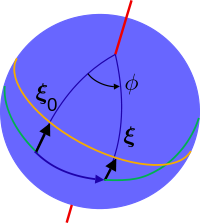
Given the mass-energy distribution provided by the stress–energy tensor T αβ, the Einstein field equations are a set of non-linear second-order partial differential equations in the metric, and imply the curvature of spacetime is equivalent to a gravitational field (see equivalence principle). Mass falling in curved spacetime is equivalent to a mass falling in a gravitational field - because gravity is a fictitious force. The relative acceleration of one geodesic to another in curved spacetime is given by the geodesic deviation equation:

where ξα = x2α − x1α is the separation vector between two geodesics, D/ds (not just d/ds) is the covariant derivative, and Rαβγδ is the Riemann curvature tensor, containing the Christoffel symbols. In other words, the geodesic deviation equation is the equation of motion for masses in curved spacetime, analogous to the Lorentz force equation for charges in an electromagnetic field.[18]: 34–35
For flat spacetime, the metric is a constant tensor so the Christoffel symbols vanish, and the geodesic equation has the solutions of straight lines. This is also the limiting case when masses move according to Newton's law of gravity.
Spinning objects edit
In general relativity, rotational motion is described by the relativistic angular momentum tensor, including the spin tensor, which enter the equations of motion under covariant derivatives with respect to proper time. The Mathisson–Papapetrou–Dixon equations describe the motion of spinning objects moving in a gravitational field.
Analogues for waves and fields edit
Unlike the equations of motion for describing particle mechanics, which are systems of coupled ordinary differential equations, the analogous equations governing the dynamics of waves and fields are always partial differential equations, since the waves or fields are functions of space and time. For a particular solution, boundary conditions along with initial conditions need to be specified.
Sometimes in the following contexts, the wave or field equations are also called "equations of motion".
Field equations edit
Equations that describe the spatial dependence and time evolution of fields are called field equations. These include
- Maxwell's equations for the electromagnetic field,
- Poisson's equation for Newtonian gravitational or electrostatic field potentials,
- the Einstein field equation for gravitation (Newton's law of gravity is a special case for weak gravitational fields and low velocities of particles).
This terminology is not universal: for example although the Navier–Stokes equations govern the velocity field of a fluid, they are not usually called "field equations", since in this context they represent the momentum of the fluid and are called the "momentum equations" instead.
Wave equations edit
Equations of wave motion are called wave equations. The solutions to a wave equation give the time-evolution and spatial dependence of the amplitude. Boundary conditions determine if the solutions describe traveling waves or standing waves.
From classical equations of motion and field equations; mechanical, gravitational wave, and electromagnetic wave equations can be derived. The general linear wave equation in 3D is:

where X = X(r, t) is any mechanical or electromagnetic field amplitude, say:[20]
- the transverse or longitudinal displacement of a vibrating rod, wire, cable, membrane etc.,
- the fluctuating pressure of a medium, sound pressure,
- the electric fields E or D, or the magnetic fields B or H,
- the voltage V or current I in an alternating current circuit,
and v is the phase velocity. Nonlinear equations model the dependence of phase velocity on amplitude, replacing v by v(X). There are other linear and nonlinear wave equations for very specific applications, see for example the Korteweg–de Vries equation.
Quantum theory edit
In quantum theory, the wave and field concepts both appear.
In quantum mechanics the analogue of the classical equations of motion (Newton's law, Euler–Lagrange equation, Hamilton–Jacobi equation, etc.) is the Schrödinger equation in its most general form:

where Ψ is the wavefunction of the system, Ĥ is the quantum Hamiltonian operator, rather than a function as in classical mechanics, and ħ is the Planck constant divided by 2π. Setting up the Hamiltonian and inserting it into the equation results in a wave equation, the solution is the wavefunction as a function of space and time. The Schrödinger equation itself reduces to the Hamilton–Jacobi equation when one considers the correspondence principle, in the limit that ħ becomes zero. To compare to measurements, operators for observables must be applied the quantum wavefunction according to the experiment performed, leading to either wave-like or particle-like results.
Throughout all aspects of quantum theory, relativistic or non-relativistic, there are various formulations alternative to the Schrödinger equation that govern the time evolution and behavior of a quantum system, for instance:
- the Heisenberg equation of motion resembles the time evolution of classical observables as functions of position, momentum, and time, if one replaces dynamical observables by their quantum operators and the classical Poisson bracket by the commutator,
- the phase space formulation closely follows classical Hamiltonian mechanics, placing position and momentum on equal footing,
- the Feynman path integral formulation extends the principle of least action to quantum mechanics and field theory, placing emphasis on the use of a Lagrangians rather than Hamiltonians.
See also edit
- Scalar (physics)
- Vector
- Distance
- Displacement
- Speed
- Velocity
- Acceleration
- Angular displacement
- Angular speed
- Angular velocity
- Angular acceleration
- Equations for a falling body
- Parabolic trajectory
- Curvilinear coordinates
- Orthogonal coordinates
- Newton's laws of motion
- Projectile motion
- Torricelli's equation
- Euler–Lagrange equation
- Generalized forces
- Newton–Euler laws of motion for a rigid body
References edit
- ^ a b R.G. Lerner; George L. Trigg (1991). Encyclopedia of Physics (second ed.). New York: VCH Publishers. ISBN 0-89573-752-3. OCLC 20853637.
- ^ a b c d Hand, Louis N.; Janet D. Finch (1998). Analytical Mechanics. Cambridge: Cambridge University Press. ISBN 978-0-521-57572-0. OCLC 37903527.
- ^ The Britannica Guide to History of Mathematics, ed. Erik Gregersen
- ^ Discourses, Galileo
- ^ Dialogues Concerning Two New Sciences, by Galileo Galilei; translated by Henry Crew, Alfonso De Salvio
- ^ Halliday, David; Resnick, Robert; Walker, Jearl (2004-06-16). Fundamentals of Physics (7 Sub ed.). Wiley. ISBN 0-471-23231-9.
- ^ a b c Forshaw, J. R.; A. Gavin Smith (2009). Dynamics and Relativity. Chichester, UK: John Wiley & Sons. ISBN 978-0-470-01460-8. OCLC 291193458.
- ^ M.R. Spiegel; S. Lipschutz; D. Spellman (2009). Vector Analysis. Schaum's Outlines (2nd ed.). McGraw Hill. p. 33. ISBN 978-0-07-161545-7.
- ^ a b Whelan, P. M.; Hodgson, M. J. (1978). Essential Principles of Physics (second ed.). London: John Murray. ISBN 0-7195-3382-1. OCLC 7102249.
- ^ Hanrahan, Val; Porkess, R (2003). Additional Mathematics for OCR. London: Hodder & Stoughton. p. 219. ISBN 0-340-86960-7.
- ^ Keith Johnson (2001). Physics for you: revised national curriculum edition for GCSE (4th ed.). Nelson Thornes. p. 135. ISBN 978-0-7487-6236-1.
The 5 symbols are remembered by "suvat". Given any three, the other two can be found.
- ^ Halpern, Alvin M. (1988). 3000 Solved Problems in Physics. Schaum Series. New York: McGraw Hill. ISBN 978-0-07-025734-4. OCLC 27398318.
- ^ a b c Kleppner, Daniel; Robert J. Kolenkow (2010). An Introduction to Mechanics. Cambridge: Cambridge University Press. ISBN 978-0-521-19821-9. OCLC 573196466.
- ^ Pain, H. J. (1983). The Physics of Vibrations and Waves (3rd ed.). Chichester [Sussex]: Wiley. ISBN 0-471-90182-2. OCLC 9392845.
- ^ R. Penrose (2007). The Road to Reality. Vintage books. p. 474. ISBN 978-0-679-77631-4.
- ^ a b c d Kibble, T. W. B. (1973). Classical Mechanics. European Physics Series (second ed.). London, UK: McGraw Hill. ISBN 0-07-084018-0. OCLC 856410.
- ^ Grant, I. S.; Phillips, W. R. (1990). Electromagnetism. Manchester Physics Series (2nd ed.). Wiley. ISBN 0-471-92712-0. OCLC 21447877.
- ^ a b J.A. Wheeler; C. Misner; K.S. Thorne (1973). Gravitation. W.H. Freeman & Co. ISBN 0-7167-0344-0.
- ^ a b C.B. Parker (1994). McGraw Hill Encyclopaedia of Physics (second ed.). ISBN 0-07-051400-3.
- ^ H.D. Young; R.A. Freedman (2008). University Physics (12th ed.). Addison-Wesley (Pearson International). ISBN 978-0-321-50130-1.