


Summary
Flux balance analysis (FBA) is a mathematical method for simulating metabolism in genome-scale reconstructions of metabolic networks. In comparison to traditional methods of modeling, FBA is less intensive in terms of the input data required for constructing the model. Simulations performed using FBA are computationally inexpensive and can calculate steady-state metabolic fluxes for large models (over 2000 reactions) in a few seconds on modern personal computers. The related method of metabolic pathway analysis seeks to find and list all possible pathways between metabolites.
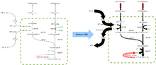
FBA finds applications in bioprocess engineering to systematically identify modifications to the metabolic networks of microbes used in fermentation processes that improve product yields of industrially important chemicals such as ethanol and succinic acid.[2] It has also been used for the identification of putative drug targets in cancer [3] and pathogens,[4] rational design of culture media,[5] and host–pathogen interactions.[6] The results of FBA can be visualized using flux maps similar to the image on the right, which illustrates the steady-state fluxes carried by reactions in glycolysis. The thickness of the arrows is proportional to the flux through the reaction.
FBA formalizes the system of equations describing the concentration changes in a metabolic network as the dot product of a matrix of the stoichiometric coefficients (the stoichiometric matrix S) and the vector v of the unsolved fluxes. The right-hand side of the dot product is a vector of zeros representing the system at steady state. Linear programming is then used to calculate a solution of fluxes corresponding to the steady state.
History edit
Some of the earliest work in FBA dates back to the early 1980s. Papoutsakis[7] demonstrated that it was possible to construct flux balance equations using a metabolic map. It was Watson,[8] however, who first introduced the idea of using linear programming and an objective function to solve for the fluxes in a pathway. The first significant study was subsequently published by Fell and Small,[9] who used flux balance analysis together with more elaborate objective functions to study the constraints in fat synthesis.
Simulations edit


FBA is not computationally intensive, taking on the order of seconds to calculate optimal fluxes for biomass production for a typical network (around 2000 reactions). This means that the effect of deleting reactions from the network and/or changing flux constraints can be sensibly modelled on a single computer.
Gene/reaction deletion and perturbation studies edit
Single reaction deletion edit
A frequently used technique to search a metabolic network for reactions that are particularly critical to the production of biomass. By removing each reaction in a network in turn and measuring the predicted flux through the biomass function, each reaction can be classified as either essential (if the flux through the biomass function is substantially reduced) or non-essential (if the flux through the biomass function is unchanged or only slightly reduced).
Pairwise reaction deletion edit
Pairwise reaction deletion of all possible pairs of reactions is useful when looking for drug targets, as it allows the simulation of multi-target treatments, either by a single drug with multiple targets or by drug combinations. Double deletion studies can also quantify the synthetic lethal interactions between different pathways providing a measure of the contribution of the pathway to overall network robustness.
Single and multiple gene deletions edit
Genes are connected to enzyme-catalyzed reactions by Boolean expressions known as Gene-Protein-Reaction expressions (GPR). Typically a GPR takes the form (Gene A AND Gene B) to indicate that the products of genes A and B are protein sub-units that assemble to form the complete protein and therefore the absence of either would result in deletion of the reaction. On the other hand, if the GPR is (Gene A OR Gene B) it implies that the products of genes A and B are isozymes. Therefore, it is possible to evaluate the effect of single or multiple gene deletions by evaluation of the GPR as a Boolean expression. If the GPR evaluates to false, the reaction is constrained to zero in the model prior to performing FBA. Thus gene knockouts can be simulated using FBA.
Interpretation of gene and reaction deletion results edit
The utility of reaction inhibition and deletion analyses becomes most apparent if a gene-protein-reaction matrix has been assembled for the network being studied with FBA. The gene-protein-reaction matrix is a binary matrix connecting genes with the proteins made from them. Using this matrix, reaction essentiality can be converted into gene essentiality indicating the gene defects which may cause a certain disease phenotype or the proteins/enzymes which are essential (and thus what enzymes are the most promising drug targets in pathogens). However, the gene-protein-reaction matrix does not specify the Boolean relationship between genes with respect to the enzyme, instead it merely indicates an association between them. Therefore, it should be used only if the Boolean GPR expression is unavailable.
Reaction inhibition edit
The effect of inhibiting a reaction, rather than removing it entirely, can be simulated in FBA by restricting the allowed flux through it. The effect of an inhibition can be classified as lethal or non-lethal by applying the same criteria as in the case of a deletion where a suitable threshold is used to distinguish “substantially reduced” from “slightly reduced”. Generally the choice of threshold is arbitrary but a reasonable estimate can be obtained from growth experiments where the simulated inhibitions/deletions are actually performed and growth rate is measured.
Growth media optimization edit
To design optimal growth media with respect to enhanced growth rates or useful by-product secretion, it is possible to use a method known as Phenotypic Phase Plane analysis. PhPP involves applying FBA repeatedly on the model while co-varying the nutrient uptake constraints and observing the value of the objective function (or by-product fluxes). PhPP makes it possible to find the optimal combination of nutrients that favor a particular phenotype or a mode of metabolism resulting in higher growth rates or secretion of industrially useful by-products. The predicted growth rates of bacteria in varying media have been shown to correlate well with experimental results,[10] as well as to define precise minimal media for the culture of Salmonella typhimurium.[11]
Host-pathogen interactions
The human microbiota is a complex system with as many as 400 trillion microbes and bacteria interacting with each other and the host. To understand key factors in this system; a multi-scale, dynamic flux-balance analysis is proposed as FBA is classified as less computationally intensive.[12]
Mathematical description edit
In contrast to the traditionally followed approach of metabolic modeling using coupled ordinary differential equations, flux balance analysis requires very little information in terms of the enzyme kinetic parameters and concentration of metabolites in the system. It achieves this by making two assumptions, steady state and optimality. The first assumption is that the modeled system has entered a steady state, where the metabolite concentrations no longer change, i.e. in each metabolite node the producing and consuming fluxes cancel each other out. The second assumption is that the organism has been optimized through evolution for some biological goal, such as optimal growth or conservation of resources. The steady-state assumption reduces the system to a set of linear equations, which is then solved to find a flux distribution that satisfies the steady-state condition subject to the stoichiometry constraints while maximizing the value of a pseudo-reaction (the objective function) representing the conversion of biomass precursors into biomass.
The steady-state assumption dates to the ideas of material balance developed to model the growth of microbial cells in fermenters in bioprocess engineering. During microbial growth, a substrate consisting of a complex mixture of carbon, hydrogen, oxygen and nitrogen sources along with trace elements are consumed to generate biomass. The material balance model for this process becomes:

If we consider the system of microbial cells to be at steady state then we may set the accumulation term to zero and reduce the material balance equations to simple algebraic equations. In such a system, substrate becomes the input to the system which is consumed and biomass is produced becoming the output from the system. The material balance may then be represented as:


Mathematically, the algebraic equations can be represented as a dot product of a matrix of coefficients and a vector of the unknowns. Since the steady-state assumption puts the accumulation term to zero. The system can be written as:

Extending this idea to metabolic networks, it is possible to represent a metabolic network as a stoichiometry balanced set of equations. Moving to the matrix formalism, we can represent the equations as the dot product of a matrix of stoichiometry coefficients (stoichiometric matrix ) and the vector of fluxes as the unknowns and set the right hand side to 0 implying the steady state.


Metabolic networks typically have more reactions than metabolites and this gives an under-determined system of linear equations containing more variables than equations. The standard approach to solve such under-determined systems is to apply linear programming.
Linear programs are problems that can be expressed in canonical form:

where x represents the vector of variables (to be determined), c and b are vectors of (known) coefficients, A is a (known) matrix of coefficients, and is the matrix transpose. The expression to be maximized or minimized is called the objective function (cTx in this case). The inequalities Ax ≤ b are the constraints which specify a convex polytope over which the objective function is to be optimized.

Linear Programming requires the definition of an objective function. The optimal solution to the LP problem is considered to be the solution which maximizes or minimizes the value of the objective function depending on the case in point. In the case of flux balance analysis, the objective function Z for the LP is often defined as biomass production. Biomass production is simulated by an equation representing a lumped reaction that converts various biomass precursors into one unit of biomass.
Therefore, the canonical form of a Flux Balance Analysis problem would be:

where represents the vector of fluxes (to be determined), is a (known) matrix of coefficients. The expression to be maximized or minimized is called the objective function ( in this case). The inequalities and define, respectively, the minimal and the maximal rates of flux for every reaction corresponding to the columns of the matrix. These rates can be experimentally determined to constrain and improve the predictive accuracy of the model even further or they can be specified to an arbitrarily high value indicating no constraint on the flux through the reaction.


The main advantage of the flux balance approach is that it does not require any knowledge of the metabolite concentrations, or more importantly, the enzyme kinetics of the system; the homeostasis assumption precludes the need for knowledge of metabolite concentrations at any time as long as that quantity remains constant, and additionally it removes the need for specific rate laws since it assumes that at steady state, there is no change in the size of the metabolite pool in the system. The stoichiometric coefficients alone are sufficient for the mathematical maximization of a specific objective function.
The objective function is essentially a measure of how each component in the system contributes to the production of the desired product. The product itself depends on the purpose of the model, but one of the most common examples is the study of total biomass. A notable example of the success of FBA is the ability to accurately predict the growth rate of the prokaryote E. coli when cultured in different conditions.[10] In this case, the metabolic system was optimized to maximize the biomass objective function. However this model can be used to optimize the production of any product, and is often used to determine the output level of some biotechnologically relevant product. The model itself can be experimentally verified by cultivating organisms using a chemostat or similar tools to ensure that nutrient concentrations are held constant. Measurements of the production of the desired objective can then be used to correct the model.
A good description of the basic concepts of FBA can be found in the freely available supplementary material to Edwards et al. 2001[10] which can be found at the Nature website.[13] Further sources include the book "Systems Biology" by B. Palsson dedicated to the subject[14] and a useful tutorial and paper by J. Orth.[15] Many other sources of information on the technique exist in published scientific literature including Lee et al. 2006,[16] Feist et al. 2008,[17] and Lewis et al. 2012.[18]
Model preparation and refinement edit
The key parts of model preparation are: creating a metabolic network without gaps, adding constraints to the model, and finally adding an objective function (often called the Biomass function), usually to simulate the growth of the organism being modelled.
Metabolic network and software tools edit

Metabolic networks can vary in scope from those describing a single pathway, up to the cell, tissue or organism. The main requirement of a metabolic network that forms the basis of an FBA-ready network is that it contains no gaps. This typically means that extensive manual curation is required, making the preparation of a metabolic network for flux-balance analysis a process that can take months or years. However, recent advances such as so-called gap-filling methods can reduce the required time to weeks or months.
Software packages for creation of FBA models include: Pathway Tools/MetaFlux,[19][20] Simpheny,[21][22] MetNetMaker,[23] COBRApy,[24] CarveMe,[25] MIOM,[26] or COBREXA.jl.[27]
Generally models are created in BioPAX or SBML format so that further analysis or visualization can take place in other software although this is not a requirement.
Constraints edit
A key part of FBA is the ability to add constraints to the flux rates of reactions within networks, forcing them to stay within a range of selected values. This lets the model more accurately simulate real metabolism. The constraints belong to two subsets from a biological perspective; boundary constraints that limit nutrient uptake/excretion and internal constraints that limit the flux through reactions within the organism. In mathematical terms, the application of constraints can be considered to reduce the solution space of the FBA model. In addition to constraints applied at the edges of a metabolic network, constraints can be applied to reactions deep within the network. These constraints are usually simple; they may constrain the direction of a reaction due to energy considerations or constrain the maximum speed of a reaction due to the finite speed of all reactions in nature.
Growth media constraints edit
Organisms, and all other metabolic systems, require some input of nutrients. Typically the rate of uptake of nutrients is dictated by their availability (a nutrient that is not present cannot be absorbed), their concentration and diffusion constants (higher concentrations of quickly-diffusing metabolites are absorbed more quickly) and the method of absorption (such as active transport or facilitated diffusion versus simple diffusion).
If the rate of absorption (and/or excretion) of certain nutrients can be experimentally measured then this information can be added as a constraint on the flux rate at the edges of a metabolic model. This ensures that nutrients that are not present or not absorbed by the organism do not enter its metabolism (the flux rate is constrained to zero) and also means that known nutrient uptake rates are adhered to by the simulation. This provides a secondary method of making sure that the simulated metabolism has experimentally verified properties rather than just mathematically acceptable ones.
Thermodynamical reaction constraints edit
In principle, all reactions are reversible however in practice reactions often effectively occur in only one direction. This may be due to significantly higher concentration of reactants compared to the concentration of the products of the reaction. But more often it happens because the products of a reaction have a much lower free energy than the reactants and therefore the forward direction of a reaction is favored more.
For ideal reactions,

For certain reactions a thermodynamic constraint can be applied implying direction (in this case forward)

Realistically the flux through a reaction cannot be infinite (given that enzymes in the real system are finite) which implies that,

Experimentally measured flux constraints edit
Certain flux rates can be measured experimentally ( ) and the fluxes within a metabolic model can be constrained, within some error ( ), to ensure these known flux rates are accurately reproduced in the simulation.


Flux rates are most easily measured for nutrient uptake at the edge of the network. Measurements of internal fluxes is possible using radioactively labelled or NMR visible metabolites.
Constrained FBA-ready metabolic models can be analyzed using software such as the COBRA toolbox[28] (available implementations in MATLAB and Python), SurreyFBA,[29] or the web-based FAME.[30] Additional software packages have been listed elsewhere.[31] A comprehensive review of all such software and their functionalities has been recently reviewed.[32]
An open-source alternative is available in the R (programming language) as the packages abcdeFBA or sybil[33] for performing FBA and other constraint based modeling techniques.[34]
Objective function edit
FBA can give a large number of mathematically acceptable solutions to the steady-state problem . However solutions of biological interest are the ones which produce the desired metabolites in the correct proportion. The objective function defines the proportion of these metabolites. For instance when modelling the growth of an organism the objective function is generally defined as biomass. Mathematically, it is a column in the stoichiometry matrix the entries of which place a "demand" or act as a "sink" for biosynthetic precursors such as fatty acids, amino acids and cell wall components which are present on the corresponding rows of the S matrix. These entries represent experimentally measured, dry weight proportions of cellular components. Therefore, this column becomes a lumped reaction that simulates growth and reproduction. Therefore, the accuracy of experimental measurements plays an essential role in the correct definition of the biomass function and makes the results of FBA biologically applicable by ensuring that the correct proportion of metabolites are produced by metabolism.

When modeling smaller networks the objective function can be changed accordingly. An example of this would be in the study of the carbohydrate metabolism pathways where the objective function would probably be defined as a certain proportion of ATP and NADH and thus simulate the production of high energy metabolites by this pathway.
Optimization of the objective/biomass function edit
Linear programming can be used to find a single optimal solution. The most common biological optimization goal for a whole-organism metabolic network would be to choose the flux vector that maximises the flux through a biomass function composed of the constituent metabolites of the organism placed into the stoichiometric matrix and denoted or simply


In the more general case any reaction can be defined and added to the biomass function with either the condition that it be maximised or minimised if a single “optimal” solution is desired. Alternatively, and in the most general case, a vector can be introduced, which defines the weighted set of reactions that the linear programming model should aim to maximise or minimise,


In the case of there being only a single separate biomass function/reaction within the stoichiometric matrix would simplify to all zeroes with a value of 1 (or any non-zero value) in the position corresponding to that biomass function. Where there were multiple separate objective functions would simplify to all zeroes with weighted values in the positions corresponding to all objective functions.
Reducing the solution space – biological considerations for the system edit
The analysis of the null space of matrices is implemented in software packages specialized for matrix operations such as Matlab and Octave. Determination of the null space of tells us all the possible collections of flux vectors (or linear combinations thereof) that balance fluxes within the biological network. The advantage of this approach becomes evident in biological systems which are described by differential equation systems with many unknowns. The velocities in the differential equations above - and - are dependent on the reaction rates of the underlying equations. The velocities are generally taken from the Michaelis–Menten kinetic theory, which involves the kinetic parameters of the enzymes catalyzing the reactions and the concentration of the metabolites themselves. Isolating enzymes from living organisms and measuring their kinetic parameters is a difficult task, as is measuring the internal concentrations and diffusion constants of metabolites within an organism. Therefore, the differential equation approach to metabolic modeling is beyond the current scope of science for all but the most studied organisms.[35] FBA avoids this impediment by applying the homeostatic assumption, which is a reasonably approximate description of biological systems.


Although FBA avoids that biological obstacle, the mathematical issue of a large solution space remains. FBA has a two-fold purpose. Accurately representing the biological limits of the system and returning the flux distribution closest to the natural fluxes within the target system/organism. Certain biological principles can help overcome the mathematical difficulties. While the stoichiometric matrix is almost always under-determined initially (meaning that the solution space to is very large), the size of the solution space can be reduced and be made more reflective of the biology of the problem through the application of certain constraints on the solutions.

Extensions edit
The success of FBA and the realization of its limitations has led to extensions that attempt to mediate the limitations of the technique.
Flux variability analysis edit

The optimal solution to the flux-balance problem is rarely unique with many possible, and equally optimal, solutions existing. Flux variability analysis (FVA), built into some analysis software, returns the boundaries for the fluxes through each reaction that can, paired with the right combination of other fluxes, estimate the optimal solution.

Reactions which can support a low variability of fluxes through them are likely to be of a higher importance to an organism and FVA is a promising technique for the identification of reactions that are important.
Minimization of metabolic adjustment (MOMA) edit
When simulating knockouts or growth on media, FBA gives the final steady-state flux distribution. This final steady state is reached in varying time-scales. For example, the predicted growth rate of E. coli on glycerol as the primary carbon source did not match the FBA predictions; however, on sub-culturing for 40 days or 700 generations, the growth rate adaptively evolved to match the FBA prediction.[36]
Sometimes it is of interest to find out what is the immediate effect of a perturbation or knockout, since it takes time for regulatory changes to occur and for the organism to re-organize fluxes to optimally utilize a different carbon source or circumvent the effect of the knockout. MOMA predicts the immediate sub-optimal flux distribution following the perturbation by minimizing the distance (Euclidean) between the wild-type FBA flux distribution and the mutant flux distribution using quadratic programming. This yields an optimization problem of the form.

where represents the wild-type (or unperturbed state) flux distribution and represents the flux distribution on gene deletion that is to be solved for. This simplifies to:


This is the MOMA solution which represents the flux distribution immediately post-perturbation.[37]
Regulatory on-off minimization (ROOM) edit
ROOM attempts to improve the prediction of the metabolic state of an organism after a gene knockout. It follows the same premise as MOMA that an organism would try to restore a flux distribution as close as possible to the wild-type after a knockout. However it further hypothesizes that this steady state would be reached through a series of transient metabolic changes by the regulatory network and that the organism would try to minimize the number of regulatory changes required to reach the wild-type state. Instead of using a distance metric minimization however it uses a mixed integer linear programming method.[38]
Dynamic FBA edit
Dynamic FBA attempts to add the ability for models to change over time, thus in some ways avoiding the strict steady state condition of pure FBA. Typically the technique involves running an FBA simulation, changing the model based on the outputs of that simulation, and rerunning the simulation. By repeating this process an element of feedback is achieved over time.
Comparison with other techniques edit
FBA provides a less simplistic analysis than Choke Point Analysis while requiring far less information on reaction rates and a much less complete network reconstruction than a full dynamic simulation would require. In filling this niche, FBA has been shown to be a very useful technique for analysis of the metabolic capabilities of cellular systems.
Choke point analysis edit
Unlike choke point analysis which only considers points in the network where metabolites are produced but not consumed or vice versa, FBA is a true form of metabolic network modelling because it considers the metabolic network as a single complete entity (the stoichiometric matrix) at all stages of analysis. This means that network effects, such as chemical reactions in distant pathways affecting each other, can be reproduced in the model. The upside to the inability of choke point analysis to simulate network effects is that it considers each reaction within a network in isolation and thus can suggest important reactions in a network even if a network is highly fragmented and contains many gaps.
Dynamic metabolic simulation edit
Unlike dynamic metabolic simulation, FBA assumes that the internal concentration of metabolites within a system stays constant over time and thus is unable to provide anything other than steady-state solutions. It is unlikely that FBA could, for example, simulate the functioning of a nerve cell. Since the internal concentration of metabolites is not considered within a model, it is possible that an FBA solution could contain metabolites at a concentration too high to be biologically acceptable. This is a problem that dynamic metabolic simulations would probably avoid. One advantage of the simplicity of FBA over dynamic simulations is that they are far less computationally expensive, allowing the simulation of large numbers of perturbations to the network. A second advantage is that the reconstructed model can be substantially simpler by avoiding the need to consider enzyme rates and the effect of complex interactions on enzyme kinetics.
See also edit
References edit
- ^ a b c d e f Forth, Thomas (2012). Metabolic systems biology of the malaria parasite. Leeds, UK: University of Leeds. ISBN 978-0-85731-297-6.
- ^ Ranganathan, Sridhar; Suthers, Patrick F.; Maranas, Costas D. (2010). "OptForce: An Optimization Procedure for Identifying All Genetic Manipulations Leading to Targeted Overproductions". PLOS Comput Biol. 6 (4): e1000744. Bibcode:2010PLSCB...6E0744R. doi:10.1371/journal.pcbi.1000744. PMC 2855329. PMID 20419153.
- ^ Lewis, NE; Abdel-Haleem, AM (2013). "The evolution of genome-scale models of cancer metabolism". Front. Physiol. 4: 237. doi:10.3389/fphys.2013.00237. PMC 3759783. PMID 24027532.
- ^ Raman, Karthik; Yeturu, Kalidas; Chandra, Nagasuma (2008). "targetTB: A Target Identification Pipeline for Mycobacterium tuberculosis Through an Interactome, Reactome and Genome-scale Structural Analysis". BMC Systems Biology. 2 (1): 109. doi:10.1186/1752-0509-2-109. PMC 2651862. PMID 19099550.
- ^ Yang, Hong; Roth, Charles M.; Ierapetritou, Marianthi G. (2009). "A rational design approach for amino acid supplementation in hepatocyte culture". Biotechnology and Bioengineering. 103 (6): 1176–1191. doi:10.1002/bit.22342. PMID 19422042. S2CID 13230467.
- ^ Raghunathan, Anu; Shin, Sookil; Daefler, Simon (2010). "Systems Approach to Investigating Host-pathogen Interactions in Infections with the Biothreat Agent Francisella. Constraints-based Model of Francisella tularensis". BMC Systems Biology. 4 (1): 118. doi:10.1186/1752-0509-4-118. PMC 2933595. PMID 20731870.
- ^ Papoutsakis, ET (1984). "Equations and calculations for fermentations of butyric acid bacteria". Biotechnology and Bioengineering. 26 (2): 174–187. doi:10.1002/bit.260260210. PMID 18551704. S2CID 25023799.
- ^ Watson MR (1984) Metabolic maps for the Apple II. 12, 1093-1094
- ^ Fell, DA; Small, JR (1986). "Fat synthesis in adipose tissue. An examination of stoichiometric constraints". Biochem J. 238 (3): 781–786. doi:10.1042/bj2380781. PMC 1147204. PMID 3800960.
- ^ a b c Edwards, J.; Ibarra, R.; Palsson, B. (2001). "In silico predictions of Escherichia coli metabolic capabilities are consistent with experimental data". Nature Biotechnology. 19 (2): 125–130. doi:10.1038/84379. PMID 11175725. S2CID 1619105.
- ^ Raghunathan, A.; et al. (2009). "Constraint-based analysis of metabolic capacity of Salmonella typhimurium during host-pathogen interaction". BMC Systems Biology. 3: 38. doi:10.1186/1752-0509-3-38. PMC 2678070. PMID 19356237.
- ^ Hoek, Milan J. A. van; Merks, Roeland M. H. (2017-05-16). "Emergence of microbial diversity due to cross-feeding interactions in a spatial model of gut microbial metabolism". BMC Systems Biology. 11 (1): 56. doi:10.1186/s12918-017-0430-4. ISSN 1752-0509. PMC 5434578. PMID 28511646.
- ^ "Archived copy". Archived from the original on 2008-02-01. Retrieved 2007-12-01.
{{cite web}}: CS1 maint: archived copy as title (link) - ^ Palsson, B.O. Systems Biology: Properties of Reconstructed Networks. 334(Cambridge University Press: 2006).
- ^ Orth, J.D.; Thiele, I.; Palsson, B.Ø. (2010). "What is flux balance analysis?". Nature Biotechnology. 28 (3): 245–248. doi:10.1038/nbt.1614. PMC 3108565. PMID 20212490.
- ^ Lee, J.M.; Gianchandani, E.P.; Papin, J.A. (2006). "Flux balance analysis in the era of metabolomics". Briefings in Bioinformatics. 7 (2): 140–50. doi:10.1093/bib/bbl007. PMID 16772264.
- ^ Feist, A.M.; Palsson, B.Ø. (2008). "The growing scope of applications of genome-scale metabolic reconstructions using Escherichia coli". Nature Biotechnology. 26 (6): 659–67. doi:10.1038/nbt1401. PMC 3108568. PMID 18536691.
- ^ Lewis, N.E.; Nagarajan, H.; Palsson, B.Ø. (2012). "Constraining the metabolic genotype–phenotype relationship using a phylogeny of in silico methods". Nature Reviews Microbiology. 10 (4): 291–305. doi:10.1038/nrmicro2737. PMC 3536058. PMID 22367118.
- ^ Karp, P.D.; Paley, S.M.; Krummenacker, M.; et al. (2010). "Pathway Tools version 13.0: Integrated Software for Pathway/Genome Informatics and Systems Biology". Briefings in Bioinformatics. 11 (1): 40–79. arXiv:1510.03964. doi:10.1093/bib/bbp043. PMC 2810111. PMID 19955237.
- ^ Latendresse, M.; Krummenacker, M.; Trupp, M.; Karp, P.D. (2012). "Construction and completion of flux balance models from pathway databases". Bioinformatics. 28 (388–96): 388–96. doi:10.1093/bioinformatics/btr681. PMC 3268246. PMID 22262672.
- ^ Schilling, C.H. et al. SimPheny: A Computational Infrastructure for Systems Biology. (2008).
- ^ "Genomatica | Technology: Technology Suite". Archived from the original on 2010-04-21. Retrieved 2010-03-11.
- ^ "MetNetMaker on Tom's Personal Page".
- ^ "COBRApy: Constraint-Based Reconstruction and Analysis in Python". GitHub. 2013.
- ^ "Genome-scale metabolic model reconstruction with CarveMe". GitHub. 28 October 2021.
- ^ "MIOM: Constraint-based modeling of metabolism using Mixed Integer Optimization". GitHub. 26 July 2021.
- ^ "Constraint-Based Reconstruction and Exascale Analysis". GitHub. 16 May 2021.
- ^ Becker, S.A.; et al. (2007). "Quantitative prediction of cellular metabolism with constraint-based models: the COBRA Toolbox". Nature Protocols. 2 (3): 727–38. doi:10.1038/nprot.2007.99. PMID 17406635. S2CID 5687582.
- ^ Gevorgyan, A; Bushell, ME; Avignone-Rossa, C; Kierzek, AM (2011). "SurreyFBA: a command line tool and graphics user interface for constraint-based modeling of genome-scale metabolic reaction networks". Bioinformatics. 27 (3): 433–4. doi:10.1093/bioinformatics/btq679. PMID 21148545.
- ^ Boele, J; Olivier, BG; Teusink, B (2012). "FAME: the Flux Analysis and Modeling Environment". BMC Syst Biol. 6 (1): 8. doi:10.1186/1752-0509-6-8. PMC 3317868. PMID 22289213.
- ^ "CoBRA Methods - Constraint-based analysis".
- ^ Lakshmanan, M; Koh, G; Chung, BK; Lee, DY (Jan 2014). "Software applications for flux balance analysis". Briefings in Bioinformatics. 15 (1): 108–22. doi:10.1093/bib/bbs069. PMID 23131418.
- ^ Gelius-Dietrich, G.; Amer Desouki, A.; Fritzemeier, C.J.; Lercher, M.J. (2013). "sybil – Efficient constraint-based modelling in R." BMC Systems Biology. 7 (1): 125. doi:10.1186/1752-0509-7-125. PMC 3843580. PMID 24224957. Software available at https://cran.r-project.org/package=sybil
- ^ Gangadharan A. Rohatgi N. abcdeFBA: Functions for Constraint Based Simulation using Flux Balance Analysis and informative analysis of the data generated during simulation. Available at: https://cran.r-project.org/web/packages/abcdeFBA/
- ^ Kotte, O.; Zaugg, J. B.; Heinemann, M. (2010). "Bacterial adaptation through distributed sensing of metabolic fluxes". Molecular Systems Biology. 6 (355): 355. doi:10.1038/msb.2010.10. PMC 2858440. PMID 20212527.
- ^ Ibarra, Rafael U.; Edwards, Jeremy S.; Palsson, Bernhard O. (2002). "Escherichia Coli K-12 Undergoes Adaptive Evolution to Achieve in Silico Predicted Optimal Growth". Nature. 420 (6912): 186–189. Bibcode:2002Natur.420..186I. doi:10.1038/nature01149. PMID 12432395. S2CID 4415915.
- ^ Segrè, Daniel; Vitkup, Dennis; Church, George M. (2002). "Analysis of Optimality in Natural and Perturbed Metabolic Networks". Proceedings of the National Academy of Sciences. 99 (23): 15112–15117. Bibcode:2002PNAS...9915112S. doi:10.1073/pnas.232349399. PMC 137552. PMID 12415116.
- ^ Shlomi, Tomer, Omer Berkman, and Eytan Ruppin. "Regulatory On/off Minimization of Metabolic Flux Changes After Genetic Perturbations." Proceedings of the National Academy of Sciences of the United States of America 102, no. 21 (May 24, 2005): 7695–7700. doi:10.1073/pnas.0406346102.