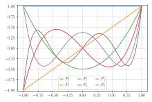
For the simplest integration problem stated above, i.e., f(x) is well-approximated by polynomials on ${\displaystyle [-1,1]}$ , the associated orthogonal polynomials are Legendre polynomials, denoted by P_n(x). With the n-th polynomial normalized to give P_n(1) = 1, the i-th Gauss node, x_i, is the i-th root of P_n and the weights are given by the formula^[3]

Some low-order quadrature rules are tabulated below (over interval [−1, 1], see the section below for other intervals).

An integral over [a, b] must be changed into an integral over [−1, 1] before applying the Gaussian quadrature rule. This change of interval can be done in the following way:

with ${\displaystyle {\frac {dx}{d\xi }}={\frac {b-a}{2}}}$ 

Applying the ${\displaystyle n}$  point Gaussian quadrature ${\displaystyle (\xi ,w)}$  rule then results in the following approximation:

Use the two-point Gauss quadrature rule to approximate the distance in meters covered by a rocket from ${\displaystyle t=8\mathrm {s} }$  to ${\displaystyle t=30\mathrm {s} ,}$  as given by

Change the limits so that one can use the weights and abscissae given in Table 1. Also, find the absolute relative true error. The true value is given as 11061.34 m.

Solution

First, changing the limits of integration from ${\displaystyle \left[8,30\right]}$  to ${\displaystyle \left[-1,1\right]}$  gives

Next, get the weighting factors and function argument values from Table 1 for the two-point rule,

• ${\displaystyle c_{1}=1.000000000}$ 
• ${\displaystyle x_{1}=-0.577350269}$ 
• ${\displaystyle c_{2}=1.000000000}$ 
• ${\displaystyle x_{2}=0.577350269}$ 

Now we can use the Gauss quadrature formula

Given that the true value is 11061.34 m, the absolute relative true error, ${\displaystyle \left|\varepsilon _{t}\right|}$  is

The integration problem can be expressed in a slightly more general way by introducing a positive weight function ω into the integrand, and allowing an interval other than [−1, 1]. That is, the problem is to calculate

Fundamental theorem edit

Let p_n be a nontrivial polynomial of degree n such that

Note that this will be true for all the orthogonal polynomials above, because each p_n is constructed to be orthogonal to the other polynomials p_j for j<n, and x^k is in the span of that set.

If we pick the n nodes x_i to be the zeros of p_n, then there exist n weights w_i which make the Gaussian quadrature computed integral exact for all polynomials h(x) of degree 2n − 1 or less. Furthermore, all these nodes x_i will lie in the open interval (a, b).^[4]

To prove the first part of this claim, let h(x) be any polynomial of degree 2n − 1 or less. Divide it by the orthogonal polynomial p_n to get

Since the remainder r(x) is of degree n − 1 or less, we can interpolate it exactly using n interpolation points with Lagrange polynomials l_i(x), where

We have

Then its integral will equal

where w_i, the weight associated with the node x_i, is defined to equal the weighted integral of l_i(x) (see below for other formulas for the weights). But all the x_i are roots of p_n, so the division formula above tells us that

This proves that for any polynomial h(x) of degree 2n − 1 or less, its integral is given exactly by the Gaussian quadrature sum.

To prove the second part of the claim, consider the factored form of the polynomial p_n. Any complex conjugate roots will yield a quadratic factor that is either strictly positive or strictly negative over the entire real line. Any factors for roots outside the interval from a to b will not change sign over that interval. Finally, for factors corresponding to roots x_i inside the interval from a to b that are of odd multiplicity, multiply p_n by one more factor to make a new polynomial

This polynomial cannot change sign over the interval from a to b because all its roots there are now of even multiplicity. So the integral

General formula for the weights edit

The weights can be expressed as

${\displaystyle w_{i}={\frac {a_{n}}{a_{n-1}}}{\frac {\int _{a}^{b}\omega (x)p_{n-1}(x)^{2}dx}{p'_{n}(x_{i})p_{n-1}(x_{i})}}}$

(1)

where ${\displaystyle a_{k}}$  is the coefficient of ${\displaystyle x^{k}}$  in ${\displaystyle p_{k}(x)}$ . To prove this, note that using Lagrange interpolation one can express r(x) in terms of ${\displaystyle r(x_{i})}$  as

The weights w_i are thus given by

This integral expression for ${\displaystyle w_{i}}$  can be expressed in terms of the orthogonal polynomials ${\displaystyle p_{n}(x)}$  and ${\displaystyle p_{n-1}(x)}$  as follows.

We can write

where ${\displaystyle a_{n}}$  is the coefficient of ${\displaystyle x^{n}}$  in ${\displaystyle p_{n}(x)}$ . Taking the limit of x to ${\displaystyle x_{i}}$  yields using L'Hôpital's rule

We can thus write the integral expression for the weights as

${\displaystyle w_{i}={\frac {1}{p'_{n}(x_{i})}}\int _{a}^{b}\omega (x){\frac {p_{n}(x)}{x-x_{i}}}dx}$

(2)

In the integrand, writing

yields

provided ${\displaystyle k\leq n}$ , because

We can evaluate the integral on the right hand side for ${\displaystyle q(x)=p_{n-1}(x)}$  as follows. Because ${\displaystyle {\frac {p_{n}(x)}{x-x_{i}}}}$  is a polynomial of degree n − 1, we have

We can then write

The term in the brackets is a polynomial of degree ${\displaystyle n-2}$ , which is therefore orthogonal to ${\displaystyle p_{n-1}(x)}$ . The integral can thus be written as

According to equation (2), the weights are obtained by dividing this by ${\displaystyle p'_{n}(x_{i})}$  and that yields the expression in equation (1).

${\displaystyle w_{i}}$  can also be expressed in terms of the orthogonal polynomials ${\displaystyle p_{n}(x)}$  and now ${\displaystyle p_{n+1}(x)}$ . In the 3-term recurrence relation ${\displaystyle p_{n+1}(x_{i})=(a)p_{n}(x_{i})+(b)p_{n-1}(x_{i})}$  the term with ${\displaystyle p_{n}(x_{i})}$  vanishes, so ${\displaystyle p_{n-1}(x_{i})}$  in Eq. (1) can be replaced by ${\textstyle {\frac {1}{b}}p_{n+1}\left(x_{i}\right)}$ .

Proof that the weights are positive edit

Consider the following polynomial of degree ${\displaystyle 2n-2}$ 

Since both ${\displaystyle \omega (x)}$  and ${\displaystyle f(x)}$  are non-negative functions, it follows that ${\displaystyle w_{i}>0}$ .

Computation of Gaussian quadrature rules edit

There are many algorithms for computing the nodes x_i and weights w_i of Gaussian quadrature rules. The most popular are the Golub-Welsch algorithm requiring O(n²) operations, Newton's method for solving ${\displaystyle p_{n}(x)=0}$  using the three-term recurrence for evaluation requiring O(n²) operations, and asymptotic formulas for large n requiring O(n) operations.

Recurrence relation edit

Orthogonal polynomials ${\displaystyle p_{r}}$  with ${\displaystyle (p_{r},p_{s})=0}$  for ${\displaystyle r\neq s}$  for a scalar product ${\displaystyle (\cdot ,\cdot )}$ , degree ${\displaystyle (p_{r})=r}$  and leading coefficient one (i.e. monic orthogonal polynomials) satisfy the recurrence relation

and scalar product defined

for ${\displaystyle r=0,1,\ldots ,n-1}$  where n is the maximal degree which can be taken to be infinity, and where ${\textstyle a_{r,s}={\frac {\left(xp_{r},p_{s}\right)}{\left(p_{s},p_{s}\right)}}}$ . First of all, the polynomials defined by the recurrence relation starting with ${\displaystyle p_{0}(x)=1}$  have leading coefficient one and correct degree. Given the starting point by ${\displaystyle p_{0}}$ , the orthogonality of ${\displaystyle p_{r}}$  can be shown by induction. For ${\displaystyle r=s=0}$  one has

Now if ${\displaystyle p_{0},p_{1},\ldots ,p_{r}}$  are orthogonal, then also ${\displaystyle p_{r+1}}$ , because in

However, if the scalar product satisfies ${\displaystyle (xf,g)=(f,xg)}$  (which is the case for Gaussian quadrature), the recurrence relation reduces to a three-term recurrence relation: For ${\displaystyle s<r-1,xp_{s}}$  is a polynomial of degree less than or equal to r − 1. On the other hand, ${\displaystyle p_{r}}$  is orthogonal to every polynomial of degree less than or equal to r − 1. Therefore, one has ${\displaystyle (xp_{r},p_{s})=(p_{r},xp_{s})=0}$  and ${\displaystyle a_{r,s}=0}$  for s < r − 1. The recurrence relation then simplifies to

or

(with the convention ${\displaystyle p_{-1}(x)\equiv 0}$ ) where

(the last because of ${\displaystyle (xp_{r},p_{r-1})=(p_{r},xp_{r-1})=(p_{r},p_{r})}$ , since ${\displaystyle xp_{r-1}}$  differs from ${\displaystyle p_{r}}$  by a degree less than r).

The Golub-Welsch algorithm edit

The three-term recurrence relation can be written in matrix form ${\displaystyle J{\tilde {P}}=x{\tilde {P}}-p_{n}(x)\mathbf {e} _{n}}$  where ${\displaystyle {\tilde {P}}={\begin{bmatrix}p_{0}(x)&p_{1}(x)&\cdots &p_{n-1}(x)\end{bmatrix}}^{\mathsf {T}}}$ , ${\displaystyle \mathbf {e} _{n}}$  is the ${\displaystyle n}$ th standard basis vector, i.e., ${\displaystyle \mathbf {e} _{n}={\begin{bmatrix}0&\cdots &0&1\end{bmatrix}}^{\mathsf {T}}}$ , and J is the following tridiagonal matrix, called the Jacobi matrix:

The zeros ${\displaystyle x_{j}}$  of the polynomials up to degree n, which are used as nodes for the Gaussian quadrature can be found by computing the eigenvalues of this matrix. This procedure is known as Golub–Welsch algorithm.

For computing the weights and nodes, it is preferable to consider the symmetric tridiagonal matrix ${\displaystyle {\mathcal {J}}}$  with elements

That is,

J and ${\displaystyle {\mathcal {J}}}$  are similar matrices and therefore have the same eigenvalues (the nodes). The weights can be computed from the corresponding eigenvectors: If ${\displaystyle \phi ^{(j)}}$  is a normalized eigenvector (i.e., an eigenvector with euclidean norm equal to one) associated with the eigenvalue x_j, the corresponding weight can be computed from the first component of this eigenvector, namely:

where ${\displaystyle \mu _{0}}$  is the integral of the weight function

See, for instance, (Gil, Segura & Temme 2007) for further details.

Error estimates edit

The error of a Gaussian quadrature rule can be stated as follows.^[5] For an integrand which has 2n continuous derivatives,

In the important special case of ω(x) = 1, we have the error estimate^[6]

Stoer and Bulirsch remark that this error estimate is inconvenient in practice, since it may be difficult to estimate the order 2n derivative, and furthermore the actual error may be much less than a bound established by the derivative. Another approach is to use two Gaussian quadrature rules of different orders, and to estimate the error as the difference between the two results. For this purpose, Gauss–Kronrod quadrature rules can be useful.

Gauss–Kronrod rules edit

If the interval [a, b] is subdivided, the Gauss evaluation points of the new subintervals never coincide with the previous evaluation points (except at zero for odd numbers), and thus the integrand must be evaluated at every point. Gauss–Kronrod rules are extensions of Gauss quadrature rules generated by adding n + 1 points to an n-point rule in such a way that the resulting rule is of order 2n + 1. This allows for computing higher-order estimates while re-using the function values of a lower-order estimate. The difference between a Gauss quadrature rule and its Kronrod extension is often used as an estimate of the approximation error.

Gauss–Lobatto rules edit

Also known as Lobatto quadrature,^[7] named after Dutch mathematician Rehuel Lobatto. It is similar to Gaussian quadrature with the following differences:

1. The integration points include the end points of the integration interval.
2. It is accurate for polynomials up to degree 2n – 3, where n is the number of integration points.^[8]

Lobatto quadrature of function f(x) on interval [−1, 1]:

Abscissas: x_i is the ${\displaystyle (i-1)}$ st zero of ${\displaystyle P'_{n-1}(x)}$ , here ${\displaystyle P_{m}(x)}$ denotes the standard Legendre polynomial of m-th degree and the dash denotes the derivative.

Weights:

Remainder:

Some of the weights are:

An adaptive variant of this algorithm with 2 interior nodes^[9] is found in GNU Octave and MATLAB as quadl and integrate.^[10][11]

Citations edit

Bibliography edit

• "Gauss quadrature formula", Encyclopedia of Mathematics, EMS Press, 2001 [1994]
• ALGLIB contains a collection of algorithms for numerical integration (in C# / C++ / Delphi / Visual Basic / etc.)
• GNU Scientific Library — includes C version of QUADPACK algorithms (see also GNU Scientific Library)
• From Lobatto Quadrature to the Euler constant e
• Gaussian Quadrature Rule of Integration – Notes, PPT, Matlab, Mathematica, Maple, Mathcad at Holistic Numerical Methods Institute
• Weisstein, Eric W. "Legendre-Gauss Quadrature". MathWorld.
• Gaussian Quadrature by Chris Maes and Anton Antonov, Wolfram Demonstrations Project.
• Tabulated weights and abscissae with Mathematica source code, high precision (16 and 256 decimal places) Legendre-Gaussian quadrature weights and abscissas, for n=2 through n=64, with Mathematica source code.
• Mathematica source code distributed under the GNU LGPL for abscissas and weights generation for arbitrary weighting functions W(x), integration domains and precisions.
• Gaussian Quadrature in Boost.Math, for arbitrary precision and approximation order
• Gauss–Kronrod Quadrature in Boost.Math
• Nodes and Weights of Gaussian quadrature