


Summary
In fluid dynamics, Green's law, named for 19th-century British mathematician George Green, is a conservation law describing the evolution of non-breaking, surface gravity waves propagating in shallow water of gradually varying depth and width. In its simplest form, for wavefronts and depth contours parallel to each other (and the coast), it states:
- or
![{\displaystyle H_{1}\,\cdot \,{\sqrt[{4}]{h_{1}}}=H_{2}\,\cdot \,{\sqrt[{4}]{h_{2}}}}](https://wikimedia.org/api/rest_v1/media/math/render/svg/1714b8d07be7a68119aadf2894c14702a98adc4b)

where and are the wave heights at two different locations – 1 and 2 respectively – where the wave passes, and and are the mean water depths at the same two locations.


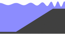
Green's law is often used in coastal engineering for the modelling of long shoaling waves on a beach, with "long" meaning wavelengths in excess of about twenty times the mean water depth.[1] Tsunamis shoal (change their height) in accordance with this law, as they propagate – governed by refraction and diffraction – through the ocean and up the continental shelf. Very close to (and running up) the coast, nonlinear effects become important and Green's law no longer applies.[2][3]
Description edit


According to this law, which is based on linearized shallow water equations, the spatial variations of the wave height (twice the amplitude for sine waves, equal to the amplitude for a solitary wave) for travelling waves in water of mean depth and width (in case of an open channel) satisfy[4][5]


![{\displaystyle H\,{\sqrt {b}}\,{\sqrt[{4}]{h}}={\text{constant}},}](https://wikimedia.org/api/rest_v1/media/math/render/svg/c6439c625dce6271d775119c0f5929d220db793a)
where is the fourth root of Consequently, when considering two cross sections of an open channel, labeled 1 and 2, the wave height in section 2 is:
![{\displaystyle {\sqrt[{4}]{h}}}](https://wikimedia.org/api/rest_v1/media/math/render/svg/3e6decf5b49fd506f06f0b5250e58db38a41efda)

![{\displaystyle H_{2}={\sqrt {\frac {b_{1}}{b_{2}}}}\;{\sqrt[{4}]{\frac {h_{1}}{h_{2}}}}\;H_{1},}](https://wikimedia.org/api/rest_v1/media/math/render/svg/acc40ddd21d2f685f1c31237da873a74a1c1afb7)
with the subscripts 1 and 2 denoting quantities in the associated cross section. So, when the depth has decreased by a factor sixteen, the waves become twice as high. And the wave height doubles after the channel width has gradually been reduced by a factor four. For wave propagation perpendicular towards a straight coast with depth contours parallel to the coastline, take a constant, say 1 metre or yard.
For refracting long waves in the ocean or near the coast, the width can be interpreted as the distance between wave rays. The rays (and the changes in spacing between them) follow from the geometrical optics approximation to the linear wave propagation.[6] In case of straight parallel depth contours this simplifies to the use of Snell's law.[7]
Green published his results in 1838,[8] based on a method – the Liouville–Green method – which would evolve into what is now known as the WKB approximation. Green's law also corresponds to constancy of the mean horizontal wave energy flux for long waves:[4][5]

where is the group speed (equal to the phase speed in shallow water), is the mean wave energy density integrated over depth and per unit of horizontal area, is the gravitational acceleration and is the water density.


Wavelength and period edit
Further, from Green's analysis, the wavelength of the wave shortens during shoaling into shallow water, with[4][8]


along a wave ray. The oscillation period (and therefore also the frequency) of shoaling waves does not change, according to Green's linear theory.
Derivation edit
Green derived his shoaling law for water waves by use of what is now known as the Liouville–Green method, applicable to gradual variations in depth and width along the path of wave propagation.[9]
Wave equation for an open channel edit
Starting point are the linearized one-dimensional Saint-Venant equations for an open channel with a rectangular cross section (vertical side walls). These equations describe the evolution of a wave with free surface elevation and horizontal flow velocity with the horizontal coordinate along the channel axis and the time:


where is the gravity of Earth (taken as a constant), is the mean water depth, is the channel width and and are denoting partial derivatives with respect to space and time. The slow variation of width and depth with distance along the channel axis is brought into account by denoting them as and where is a small parameter: The above two equations can be combined into one wave equation for the surface elevation:


-
and with the velocity following from(1)


In the Liouville–Green method, the approach is to convert the above wave equation with non-homogeneous coefficients into a homogeneous one (neglecting some small remainders in terms of ).
Transformation to the wave phase as independent variable edit
The next step is to apply a coordinate transformation, introducing the travel time (or wave phase) given by

- so


and are related through the celerity Introducing the slow variable and denoting derivatives of and with respect to with a prime, e.g. the -derivatives in the wave equation, Eq. (1), become:


Now the wave equation (1) transforms into:
-
(2)

The next step is transform the equation in such a way that only deviations from homogeneity in the second order of approximation remain, i.e. proportional to

Further transformation towards homogeneity edit
The homogeneous wave equation (i.e. Eq. (2) when is zero) has solutions for travelling waves of permanent form propagating in either the negative or positive -direction. For the inhomogeneous case, considering waves propagating in the positive -direction, Green proposes an approximate solution:

-
(3)

Then

Now the left-hand side of Eq. (2) becomes:

So the proposed solution in Eq. (3) satisfies Eq. (2), and thus also Eq. (1) apart from the above two terms proportional to and , with The error in the solution can be made of order provided


This has the solution:

Using Eq. (3) and the transformation from to , the approximate solution for the surface elevation is
-
(4)

where the constant has been set to one, without loss of generality. Waves travelling in the negative -direction have the minus sign in the argument of function reversed to a plus sign. Since the theory is linear, solutions can be added because of the superposition principle.


Sinusoidal waves and Green's law edit
Waves varying sinusoidal in time, with period are considered. That is


where is the amplitude, is the wave height, is the angular frequency and is the wave phase. Consequently, also in Eq. (4) has to be a sine wave, e.g. with a constant.


Applying these forms of and in Eq. (4) gives:


which is Green's law.
Flow velocity edit
The horizontal flow velocity in the -direction follows directly from substituting the solution for the surface elevation from Eq. (4) into the expression for in Eq. (1):[10]


and an additional constant discharge.

Note that – when the width and depth are not constants – the term proportional to implies an (small) phase difference between elevation and velocity .


For sinusoidal waves with velocity amplitude the flow velocities shoal to leading order as[8]


This could have been anticipated since for a horizontal bed with the wave amplitude.

Notes edit
- ^ Dean & Dalrymple (1991, §3.4)
- ^ Synolakis & Skjelbreia (1993)
- ^ Synolakis (1991)
- ^ a b c Lamb (1993, §185)
- ^ a b Dean & Dalrymple (1991, §5.3)
- ^ Satake (2002)
- ^ Dean & Dalrymple (1991, §4.8.2)
- ^ a b c Green (1838)
- ^ The derivation presented below is according to the line of reasoning as used by Lamb (1993, §169 & §185).
- ^ Didenkulova, Pelinovsky & Soomere (2009)
References edit
Green edit
Others edit
- Craik, A. D. D. (2004), "The origins of water wave theory", Annual Review of Fluid Mechanics, 36: 1–28, Bibcode:2004AnRFM..36....1C, doi:10.1146/annurev.fluid.36.050802.122118
- Dean, R. G.; Dalrymple, R. A. (1991), Water wave mechanics for engineers and scientists, Advanced Series on Ocean Engineering, vol. 2, World Scientific, ISBN 978-981-02-0420-4
- Didenkulova, I.; Pelinovsky, E.; Soomere, T. (2009), "Long surface wave dynamics along a convex bottom", Journal of Geophysical Research, 114 (C7): C07006, 14 pp, arXiv:0804.4369, Bibcode:2009JGRC..114.7006D, doi:10.1029/2008JC005027, S2CID 55186672
- Lamb, H. (1993), Hydrodynamics (6th ed.), Dover, ISBN 0-486-60256-7
- Satake, K. (2002), "28 – Tsunamis", in Lee, W. H. K.; Kanamori, H.; Jennings, P. C.; Kisslinger, C. (eds.), International Handbook of Earthquake and Engineering Seismology, International Geophysics, vol. 81, Part A, Academic Press, pp. 437–451, ISBN 978-0-12-440652-0
- Synolakis, C. E. (1991), "Tsunami runup on steep slopes: How good linear theory really is", Natural Hazards, 4 (2): 221–234, doi:10.1007/BF00162789, S2CID 129683723
- Synolakis, C. E.; Skjelbreia, J. E. (1993), "Evolution of maximum amplitude of solitary waves on plane beaches", Journal of Waterway, Port, Coastal, and Ocean Engineering, 119 (3): 323–342, doi:10.1061/(ASCE)0733-950X(1993)119:3(323)