


Summary
In mathematics, hyperbolic geometry (also called Lobachevskian geometry or Bolyai–Lobachevskian geometry) is a non-Euclidean geometry. The parallel postulate of Euclidean geometry is replaced with:

- For any given line R and point P not on R, in the plane containing both line R and point P there are at least two distinct lines through P that do not intersect R.
(Compare the above with Playfair's axiom, the modern version of Euclid's parallel postulate.)
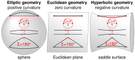
The hyperbolic plane is a plane where every point is a saddle point. Hyperbolic plane geometry is also the geometry of pseudospherical surfaces, surfaces with a constant negative Gaussian curvature. Saddle surfaces have negative Gaussian curvature in at least some regions, where they locally resemble the hyperbolic plane.
A modern use of hyperbolic geometry is in the theory of special relativity, particularly the Minkowski model.
When geometers first realised they were working with something other than the standard Euclidean geometry, they described their geometry under many different names; Felix Klein finally gave the subject the name hyperbolic geometry to include it in the now rarely used sequence elliptic geometry (spherical geometry), parabolic geometry (Euclidean geometry), and hyperbolic geometry. In the former Soviet Union, it is commonly called Lobachevskian geometry, named after one of its discoverers, the Russian geometer Nikolai Lobachevsky.
This page is mainly about the 2-dimensional (planar) hyperbolic geometry and the differences and similarities between Euclidean and hyperbolic geometry. See hyperbolic space for more information on hyperbolic geometry extended to three and more dimensions.
Properties edit
Relation to Euclidean geometry edit
Hyperbolic geometry is more closely related to Euclidean geometry than it seems: the only axiomatic difference is the parallel postulate. When the parallel postulate is removed from Euclidean geometry the resulting geometry is absolute geometry. There are two kinds of absolute geometry, Euclidean and hyperbolic. All theorems of absolute geometry, including the first 28 propositions of book one of Euclid's Elements, are valid in Euclidean and hyperbolic geometry. Propositions 27 and 28 of Book One of Euclid's Elements prove the existence of parallel/non-intersecting lines.
This difference also has many consequences: concepts that are equivalent in Euclidean geometry are not equivalent in hyperbolic geometry; new concepts need to be introduced. Further, because of the angle of parallelism, hyperbolic geometry has an absolute scale, a relation between distance and angle measurements.
Lines edit
Single lines in hyperbolic geometry have exactly the same properties as single straight lines in Euclidean geometry. For example, two points uniquely define a line, and line segments can be infinitely extended.
Two intersecting lines have the same properties as two intersecting lines in Euclidean geometry. For example, two distinct lines can intersect in no more than one point, intersecting lines form equal opposite angles, and adjacent angles of intersecting lines are supplementary.
When a third line is introduced, then there can be properties of intersecting lines that differ from intersecting lines in Euclidean geometry. For example, given two intersecting lines there are infinitely many lines that do not intersect either of the given lines.
These properties are all independent of the model used, even if the lines may look radically different.
Non-intersecting / parallel lines edit
Non-intersecting lines in hyperbolic geometry also have properties that differ from non-intersecting lines in Euclidean geometry:
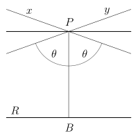
- For any line R and any point P which does not lie on R, in the plane containing line R and point P there are at least two distinct lines through P that do not intersect R.
This implies that there are through P an infinite number of coplanar lines that do not intersect R.
These non-intersecting lines are divided into two classes:
- Two of the lines (x and y in the diagram) are limiting parallels (sometimes called critically parallel, horoparallel or just parallel): there is one in the direction of each of the ideal points at the "ends" of R, asymptotically approaching R, always getting closer to R, but never meeting it.
- All other non-intersecting lines have a point of minimum distance and diverge from both sides of that point, and are called ultraparallel, diverging parallel or sometimes non-intersecting.
Some geometers simply use the phrase "parallel lines" to mean "limiting parallel lines", with ultraparallel lines meaning just non-intersecting.
These limiting parallels make an angle θ with PB; this angle depends only on the Gaussian curvature of the plane and the distance PB and is called the angle of parallelism.
For ultraparallel lines, the ultraparallel theorem states that there is a unique line in the hyperbolic plane that is perpendicular to each pair of ultraparallel lines.
Circles and disks edit
In hyperbolic geometry, the circumference of a circle of radius r is greater than .

Let , where is the Gaussian curvature of the plane. In hyperbolic geometry, is negative, so the square root is of a positive number.


Then the circumference of a circle of radius r is equal to:

And the area of the enclosed disk is:

Therefore, in hyperbolic geometry the ratio of a circle's circumference to its radius is always strictly greater than , though it can be made arbitrarily close by selecting a small enough circle.

If the Gaussian curvature of the plane is −1 then the geodesic curvature of a circle of radius r is: [1]

Hypercycles and horocycles edit

In hyperbolic geometry, there is no line all of whose points are equidistant from another line. Instead, the points that all have the same orthogonal distance from a given line lie on a curve called a hypercycle.
Another special curve is the horocycle, a curve whose normal radii (perpendicular lines) are all limiting parallel to each other (all converge asymptotically in one direction to the same ideal point, the centre of the horocycle).
Through every pair of points there are two horocycles. The centres of the horocycles are the ideal points of the perpendicular bisector of the line-segment between them.
Given any three distinct points, they all lie on either a line, hypercycle, horocycle, or circle.
The length of the line-segment is the shortest length between two points. The arc-length of a hypercycle connecting two points is longer than that of the line segment and shorter than that of a horocycle, connecting the same two points. The arclength of both horocycles connecting two points are equal. The arc-length of a circle between two points is larger than the arc-length of a horocycle connecting two points.
If the Gaussian curvature of the plane is −1 then the geodesic curvature of a horocycle is 1 and of a hypercycle is between 0 and 1.[1]
Triangles edit
Unlike Euclidean triangles, where the angles always add up to π radians (180°, a straight angle), in hyperbolic geometry the sum of the angles of a hyperbolic triangle is always strictly less than π radians (180°, a straight angle). The difference is referred to as the defect.
The area of a hyperbolic triangle is given by its defect in radians multiplied by R2. As a consequence, all hyperbolic triangles have an area that is less than or equal to R2π. The area of a hyperbolic ideal triangle in which all three angles are 0° is equal to this maximum.
As in Euclidean geometry, each hyperbolic triangle has an incircle. In hyperbolic geometry, if all three of its vertices lie on a horocycle or hypercycle, then the triangle has no circumscribed circle.
As in spherical and elliptical geometry, in hyperbolic geometry if two triangles are similar, they must be congruent.
Regular apeirogon and pseudogon edit

Special polygons in hyperbolic geometry are the regular apeirogon and pseudogon uniform polygons with an infinite number of sides.
In Euclidean geometry, the only way to construct such a polygon is to make the side lengths tend to zero and the apeirogon is indistinguishable from a circle, or make the interior angles tend to 180 degrees and the apeirogon approaches a straight line.
However, in hyperbolic geometry, a regular apeirogon or pseudogon has sides of any length (i.e., it remains a polygon with noticeable sides).
The side and angle bisectors will, depending on the side length and the angle between the sides, be limiting or diverging parallel (see lines above). If the bisectors are limiting parallel then it is an apeirogon and can be inscribed and circumscribed by concentric horocycles.
If the bisectors are diverging parallel then it is a pseudogon and can be inscribed and circumscribed by hypercycles (all vertices are the same distance of a line, the axis, also the midpoint of the side segments are all equidistant to the same axis.)
Tessellations edit

Like the Euclidean plane it is also possible to tessellate the hyperbolic plane with regular polygons as faces.
There are an infinite number of uniform tilings based on the Schwarz triangles (p q r) where 1/p + 1/q + 1/r < 1, where p, q, r are each orders of reflection symmetry at three points of the fundamental domain triangle, the symmetry group is a hyperbolic triangle group. There are also infinitely many uniform tilings that cannot be generated from Schwarz triangles, some for example requiring quadrilaterals as fundamental domains.[2]
Standardized Gaussian curvature edit
Though hyperbolic geometry applies for any surface with a constant negative Gaussian curvature, it is usual to assume a scale in which the curvature K is −1.
This results in some formulas becoming simpler. Some examples are:
- The area of a triangle is equal to its angle defect in radians.
- The area of a horocyclic sector is equal to the length of its horocyclic arc.
- An arc of a horocycle so that a line that is tangent at one endpoint is limiting parallel to the radius through the other endpoint has a length of 1.[3]
- The ratio of the arc lengths between two radii of two concentric horocycles where the horocycles are a distance 1 apart is e : 1.[3]
Cartesian-like coordinate systems edit
Compared to Euclidean geometry, hyperbolic geometry presents numerous difficulties for a coordinate system: the sum of the angles of a quadrilateral is always less than 360 degrees; there are no equidistant lines, so a proper Euclidean rectangle would need to be enclosed by two lines and two hypercycles; parallel-transporting a line segment around a quadrilateral causes it to rotate when it returns to the origin; etc.
There are however different coordinate systems for hyperbolic plane geometry. All are based around choosing a point (the origin) on a chosen directed line (the x-axis) and after that many choices exist.
The Lobachevski coordinates x and y are found by dropping a perpendicular onto the x-axis. x will be the label of the foot of the perpendicular. y will be the distance along the perpendicular of the given point from its foot (positive on one side and negative on the other).
Another coordinate system measures the distance from the point to the horocycle through the origin centered around and the length along this horocycle.[4]

Other coordinate systems use the Klein model or the Poincare disk model described below, and take the Euclidean coordinates as hyperbolic.
Distance edit
A Cartesian-like[citation needed] coordinate system (x, y) on the oriented hyperbolic plane is constructed as follows. Choose a line in the hyperbolic plane together with an orientation and an origin o on this line. Then:
- the x-coordinate of a point is the signed distance of its projection onto the line (the foot of the perpendicular segment to the line from that point) to the origin;
- the y-coordinate is the signed distance from the point to the line, with the sign according to whether the point is on the positive or negative side of the oriented line.
The distance between two points represented by (x_i, y_i), i=1,2 in this coordinate system is[citation needed]

This formula can be derived from the formulas about hyperbolic triangles.
The corresponding metric tensor field is: .

In this coordinate system, straight lines take one of these forms ((x, y) is a point on the line; x0, y0, A, and α are parameters):
ultraparallel to the x-axis

asymptotically parallel on the negative side

asymptotically parallel on the positive side

intersecting perpendicularly

intersecting at an angle α

Generally, these equations will only hold in a bounded domain (of x values). At the edge of that domain, the value of y blows up to ±infinity. See also Coordinate systems for the hyperbolic plane#Polar coordinate system.
History edit
Since the publication of Euclid's Elements circa 300 BCE, many geometers made attempts to prove the parallel postulate. Some tried to prove it by assuming its negation and trying to derive a contradiction. Foremost among these were Proclus, Ibn al-Haytham (Alhacen), Omar Khayyám,[5] Nasīr al-Dīn al-Tūsī, Witelo, Gersonides, Alfonso, and later Giovanni Gerolamo Saccheri, John Wallis, Johann Heinrich Lambert, and Legendre.[6] Their attempts were doomed to failure (as we now know, the parallel postulate is not provable from the other postulates), but their efforts led to the discovery of hyperbolic geometry.
The theorems of Alhacen, Khayyam and al-Tūsī on quadrilaterals, including the Ibn al-Haytham–Lambert quadrilateral and Khayyam–Saccheri quadrilateral, were the first theorems on hyperbolic geometry. Their works on hyperbolic geometry had a considerable influence on its development among later European geometers, including Witelo, Gersonides, Alfonso, John Wallis and Saccheri.[7]
In the 18th century, Johann Heinrich Lambert introduced the hyperbolic functions[8] and computed the area of a hyperbolic triangle.[9]
19th-century developments edit
In the 19th century, hyperbolic geometry was explored extensively by Nikolai Ivanovich Lobachevsky, János Bolyai, Carl Friedrich Gauss and Franz Taurinus. Unlike their predecessors, who just wanted to eliminate the parallel postulate from the axioms of Euclidean geometry, these authors realized they had discovered a new geometry.[10][11] Gauss wrote in an 1824 letter to Franz Taurinus that he had constructed it, but Gauss did not publish his work. Gauss called it "non-Euclidean geometry"[12] causing several modern authors to continue to consider "non-Euclidean geometry" and "hyperbolic geometry" to be synonyms. Taurinus published results on hyperbolic trigonometry in 1826, argued that hyperbolic geometry is self consistent, but still believed in the special role of Euclidean geometry. The complete system of hyperbolic geometry was published by Lobachevsky in 1829/1830, while Bolyai discovered it independently and published in 1832.
In 1868, Eugenio Beltrami provided models (see below) of hyperbolic geometry, and used this to prove that hyperbolic geometry was consistent if and only if Euclidean geometry was.
The term "hyperbolic geometry" was introduced by Felix Klein in 1871.[13] Klein followed an initiative of Arthur Cayley to use the transformations of projective geometry to produce isometries. The idea used a conic section or quadric to define a region, and used cross ratio to define a metric. The projective transformations that leave the conic section or quadric stable are the isometries. "Klein showed that if the Cayley absolute is a real curve then the part of the projective plane in its interior is isometric to the hyperbolic plane..."[14]
For more history, see article on non-Euclidean geometry, and the references Coxeter[15] and Milnor.[16]
Philosophical consequences edit
The discovery of hyperbolic geometry had important philosophical consequences. Before its discovery many philosophers (for example Hobbes and Spinoza) viewed philosophical rigour in terms of the "geometrical method", referring to the method of reasoning used in Euclid's Elements.
Kant in the Critique of Pure Reason came to the conclusion that space (in Euclidean geometry) and time are not discovered by humans as objective features of the world, but are part of an unavoidable systematic framework for organizing our experiences.[17]
It is said that Gauss did not publish anything about hyperbolic geometry out of fear of the "uproar of the Boeotians", which would ruin his status as princeps mathematicorum (Latin, "the Prince of Mathematicians").[18] The "uproar of the Boeotians" came and went, and gave an impetus to great improvements in mathematical rigour, analytical philosophy and logic. Hyperbolic geometry was finally proved consistent and is therefore another valid geometry.
Geometry of the universe (spatial dimensions only) edit
Because Euclidean, hyperbolic and elliptic geometry are all consistent, the question arises: which is the real geometry of space, and if it is hyperbolic or elliptic, what is its curvature?
Lobachevsky had already tried to measure the curvature of the universe by measuring the parallax of Sirius and treating Sirius as the ideal point of an angle of parallelism. He realised that his measurements were not precise enough to give a definite answer, but he did reach the conclusion that if the geometry of the universe is hyperbolic, then the absolute length is at least one million times the diameter of the Earth's orbit (2000000 AU, 10 parsec).[19] Some argue that his measurements were methodologically flawed.[20]
Henri Poincaré, with his sphere-world thought experiment, came to the conclusion that everyday experience does not necessarily rule out other geometries.
The geometrization conjecture gives a complete list of eight possibilities for the fundamental geometry of our space. The problem in determining which one applies is that, to reach a definitive answer, we need to be able to look at extremely large shapes – much larger than anything on Earth or perhaps even in our galaxy.[21]
Geometry of the universe (special relativity) edit
Special relativity places space and time on equal footing, so that one considers the geometry of a unified spacetime instead of considering space and time separately.[22][23] Minkowski geometry replaces Galilean geometry (which is the three-dimensional Euclidean space with time of Galilean relativity).[24]
In relativity, rather than considering Euclidean, elliptic and hyperbolic geometries, the appropriate geometries to consider are Minkowski space, de Sitter space and anti-de Sitter space,[25][26] corresponding to zero, positive and negative curvature respectively.
Hyperbolic geometry enters special relativity through rapidity, which stands in for velocity, and is expressed by a hyperbolic angle. The study of this velocity geometry has been called kinematic geometry. The space of relativistic velocities has a three-dimensional hyperbolic geometry, where the distance function is determined from the relative velocities of "nearby" points (velocities).[27]
Physical realizations of the hyperbolic plane edit


There exist various pseudospheres in Euclidean space that have a finite area of constant negative Gaussian curvature.
By Hilbert's theorem, it is not possible to isometrically immerse a complete hyperbolic plane (a complete regular surface of constant negative Gaussian curvature) in a three-dimensional Euclidean space.
Other useful models of hyperbolic geometry exist in Euclidean space, in which the metric is not preserved. A particularly well-known paper model based on the pseudosphere is due to William Thurston.
The art of crochet has been used (see Mathematics and fiber arts § Knitting and crochet) to demonstrate hyperbolic planes, the first such demonstration having been made by Daina Taimiņa.[28]
In 2000, Keith Henderson demonstrated a quick-to-make paper model dubbed the "hyperbolic soccerball" (more precisely, a truncated order-7 triangular tiling).[29][30]
Instructions on how to make a hyperbolic quilt, designed by Helaman Ferguson,[31] have been made available by Jeff Weeks.[32]
Models of the hyperbolic plane edit
Various pseudospheres – surfaces with constant negative Gaussian curvature – can be embedded in 3-dimensional space under the standard Euclidean metric, and so can be made into tangible physical models. Of these, the tractoid (often called the pseudosphere) is the best known; using the tractoid as a model of the hyperbolic plane is analogous to using a cone or cylinder as a model of the Euclidean plane. However, the entire hyperbolic plane cannot be embedded into Euclidean space in this way, and various other models are more convenient for abstractly exploring hyperbolic geometry.
There are four models commonly used for hyperbolic geometry: the Klein model, the Poincaré disk model, the Poincaré half-plane model, and the Lorentz or hyperboloid model. These models define a hyperbolic plane which satisfies the axioms of a hyperbolic geometry. Despite their names, the first three mentioned above were introduced as models of hyperbolic space by Beltrami, not by Poincaré or Klein. All these models are extendable to more dimensions.
The Beltrami–Klein model edit
The Beltrami–Klein model, also known as the projective disk model, Klein disk model and Klein model, is named after Eugenio Beltrami and Felix Klein.
For the two dimensions this model uses the interior of the unit circle for the complete hyperbolic plane, and the chords of this circle are the hyperbolic lines.
For higher dimensions this model uses the interior of the unit ball, and the chords of this n-ball are the hyperbolic lines.
- This model has the advantage that lines are straight, but the disadvantage that angles are distorted (the mapping is not conformal), and also circles are not represented as circles.
- The distance in this model is half the logarithm of the cross-ratio, which was introduced by Arthur Cayley in projective geometry.
The Poincaré disk model edit

The Poincaré disk model, also known as the conformal disk model, also employs the interior of the unit circle, but lines are represented by arcs of circles that are orthogonal to the boundary circle, plus diameters of the boundary circle.
- This model preserves angles, and is thereby conformal. All isometries within this model are therefore Möbius transformations.
- Circles entirely within the disk remain circles although the Euclidean center of the circle is closer to the center of the disk than is the hyperbolic center of the circle.
- Horocycles are circles within the disk which are tangent to the boundary circle, minus the point of contact.
- Hypercycles are open-ended chords and circular arcs within the disc that terminate on the boundary circle at non-orthogonal angles.
The Poincaré half-plane model edit
The Poincaré half-plane model takes one-half of the Euclidean plane, bounded by a line B of the plane, to be a model of the hyperbolic plane. The line B is not included in the model.
The Euclidean plane may be taken to be a plane with the Cartesian coordinate system and the x-axis is taken as line B and the half plane is the upper half (y > 0 ) of this plane.
- Hyperbolic lines are then either half-circles orthogonal to B or rays perpendicular to B.
- The length of an interval on a ray is given by logarithmic measure so it is invariant under a homothetic transformation
- Like the Poincaré disk model, this model preserves angles, and is thus conformal. All isometries within this model are therefore Möbius transformations of the plane.
- The half-plane model is the limit of the Poincaré disk model whose boundary is tangent to B at the same point while the radius of the disk model goes to infinity.

The hyperboloid model edit
The hyperboloid model or Lorentz model employs a 2-dimensional hyperboloid of revolution (of two sheets, but using one) embedded in 3-dimensional Minkowski space. This model is generally credited to Poincaré, but Reynolds[33] says that Wilhelm Killing used this model in 1885
- This model has direct application to special relativity, as Minkowski 3-space is a model for spacetime, suppressing one spatial dimension. One can take the hyperboloid to represent the events (positions in spacetime) that various inertially moving observers, starting from a common event, will reach in a fixed proper time.
- The hyperbolic distance between two points on the hyperboloid can then be identified with the relative rapidity between the two corresponding observers.
- The model generalizes directly to an additional dimension: a hyperbolic 3-space three-dimensional hyperbolic geometry relates to Minkowski 4-space.
The hemisphere model edit
The hemisphere model is not often used as model by itself, but it functions as a useful tool for visualising transformations between the other models.
The hemisphere model uses the upper half of the unit sphere:

The hyperbolic lines are half-circles orthogonal to the boundary of the hemisphere.
The hemisphere model is part of a Riemann sphere, and different projections give different models of the hyperbolic plane:
- Stereographic projection from onto the plane projects corresponding points on the Poincaré disk model
- Stereographic projection from onto the surface projects corresponding points on the hyperboloid model
- Stereographic projection from onto the plane projects corresponding points on the Poincaré half-plane model
- Orthographic projection onto a plane projects corresponding points on the Beltrami–Klein model.
- Central projection from the centre of the sphere onto the plane projects corresponding points on the Gans Model


See further: Connection between the models (below)
The Gans model edit
In 1966 David Gans proposed a flattened hyperboloid model in the journal American Mathematical Monthly.[34] It is an orthographic projection of the hyperboloid model onto the xy-plane. This model is not as widely used as other models but nevertheless is quite useful in the understanding of hyperbolic geometry.
- Unlike the Klein or the Poincaré models, this model utilizes the entire Euclidean plane.
- The lines in this model are represented as branches of a hyperbola.[35]
The band model edit
The band model employs a portion of the Euclidean plane between two parallel lines.[36] Distance is preserved along one line through the middle of the band. Assuming the band is given by , the metric is given by .


Connection between the models edit

All models essentially describe the same structure. The difference between them is that they represent different coordinate charts laid down on the same metric space, namely the hyperbolic plane. The characteristic feature of the hyperbolic plane itself is that it has a constant negative Gaussian curvature, which is indifferent to the coordinate chart used. The geodesics are similarly invariant: that is, geodesics map to geodesics under coordinate transformation. Hyperbolic geometry generally is introduced in terms of the geodesics and their intersections on the hyperbolic plane.[37]
Once we choose a coordinate chart (one of the "models"), we can always embed it in a Euclidean space of same dimension, but the embedding is clearly not isometric (since the curvature of Euclidean space is 0). The hyperbolic space can be represented by infinitely many different charts; but the embeddings in Euclidean space due to these four specific charts show some interesting characteristics.
Since the four models describe the same metric space, each can be transformed into the other.
See, for example:
Isometries of the hyperbolic plane edit
Every isometry (transformation or motion) of the hyperbolic plane to itself can be realized as the composition of at most three reflections. In n-dimensional hyperbolic space, up to n+1 reflections might be required. (These are also true for Euclidean and spherical geometries, but the classification below is different.)
All the isometries of the hyperbolic plane can be classified into these classes:
- Orientation preserving
- the identity isometry — nothing moves; zero reflections; zero degrees of freedom.
- inversion through a point (half turn) — two reflections through mutually perpendicular lines passing through the given point, i.e. a rotation of 180 degrees around the point; two degrees of freedom.
- rotation around a normal point — two reflections through lines passing through the given point (includes inversion as a special case); points move on circles around the center; three degrees of freedom.
- "rotation" around an ideal point (horolation) — two reflections through lines leading to the ideal point; points move along horocycles centered on the ideal point; two degrees of freedom.
- translation along a straight line — two reflections through lines perpendicular to the given line; points off the given line move along hypercycles; three degrees of freedom.
- Orientation reversing
- reflection through a line — one reflection; two degrees of freedom.
- combined reflection through a line and translation along the same line — the reflection and translation commute; three reflections required; three degrees of freedom.[citation needed]
Hyperbolic geometry in art edit
M. C. Escher's famous prints Circle Limit III and Circle Limit IV illustrate the conformal disc model (Poincaré disk model) quite well. The white lines in III are not quite geodesics (they are hypercycles), but are close to them. It is also possible to see quite plainly the negative curvature of the hyperbolic plane, through its effect on the sum of angles in triangles and squares.
For example, in Circle Limit III every vertex belongs to three triangles and three squares. In the Euclidean plane, their angles would sum to 450°; i.e., a circle and a quarter. From this, we see that the sum of angles of a triangle in the hyperbolic plane must be smaller than 180°. Another visible property is exponential growth. In Circle Limit III, for example, one can see that the number of fishes within a distance of n from the center rises exponentially. The fishes have an equal hyperbolic area, so the area of a ball of radius n must rise exponentially in n.
The art of crochet has been used to demonstrate hyperbolic planes (pictured above) with the first being made by Daina Taimiņa,[28] whose book Crocheting Adventures with Hyperbolic Planes won the 2009 Bookseller/Diagram Prize for Oddest Title of the Year.[38]
HyperRogue is a roguelike game set on various tilings of the hyperbolic plane.
Higher dimensions edit
Hyperbolic geometry is not limited to 2 dimensions; a hyperbolic geometry exists for every higher number of dimensions.
Homogeneous structure edit
Hyperbolic space of dimension n is a special case of a Riemannian symmetric space of noncompact type, as it is isomorphic to the quotient

The orthogonal group O(1, n) acts by norm-preserving transformations on Minkowski space R1,n, and it acts transitively on the two-sheet hyperboloid of norm 1 vectors. Timelike lines (i.e., those with positive-norm tangents) through the origin pass through antipodal points in the hyperboloid, so the space of such lines yields a model of hyperbolic n-space. The stabilizer of any particular line is isomorphic to the product of the orthogonal groups O(n) and O(1), where O(n) acts on the tangent space of a point in the hyperboloid, and O(1) reflects the line through the origin. Many of the elementary concepts in hyperbolic geometry can be described in linear algebraic terms: geodesic paths are described by intersections with planes through the origin, dihedral angles between hyperplanes can be described by inner products of normal vectors, and hyperbolic reflection groups can be given explicit matrix realizations.
In small dimensions, there are exceptional isomorphisms of Lie groups that yield additional ways to consider symmetries of hyperbolic spaces. For example, in dimension 2, the isomorphisms SO+(1, 2) ≅ PSL(2, R) ≅ PSU(1, 1) allow one to interpret the upper half plane model as the quotient SL(2, R)/SO(2) and the Poincaré disc model as the quotient SU(1, 1)/U(1). In both cases, the symmetry groups act by fractional linear transformations, since both groups are the orientation-preserving stabilizers in PGL(2, C) of the respective subspaces of the Riemann sphere. The Cayley transformation not only takes one model of the hyperbolic plane to the other, but realizes the isomorphism of symmetry groups as conjugation in a larger group. In dimension 3, the fractional linear action of PGL(2, C) on the Riemann sphere is identified with the action on the conformal boundary of hyperbolic 3-space induced by the isomorphism O+(1, 3) ≅ PGL(2, C). This allows one to study isometries of hyperbolic 3-space by considering spectral properties of representative complex matrices. For example, parabolic transformations are conjugate to rigid translations in the upper half-space model, and they are exactly those transformations that can be represented by unipotent upper triangular matrices.
See also edit
- Band model
- Constructions in hyperbolic geometry
- Hjelmslev transformation
- Hyperbolic 3-manifold
- Hyperbolic manifold
- Hyperbolic set
- Hyperbolic tree
- Kleinian group
- Lambert quadrilateral
- Open universe
- Poincaré metric
- Saccheri quadrilateral
- Systolic geometry
- Uniform tilings in hyperbolic plane
- δ-hyperbolic space
Notes edit
- ^ a b "Curvature of curves on the hyperbolic plane". math stackexchange. Retrieved 24 September 2017.
- ^ Hyde, S.T.; Ramsden, S. (2003). "Some novel three-dimensional Euclidean crystalline networks derived from two-dimensional hyperbolic tilings". The European Physical Journal B. 31 (2): 273–284. Bibcode:2003EPJB...31..273H. CiteSeerX 10.1.1.720.5527. doi:10.1140/epjb/e2003-00032-8. S2CID 41146796.
- ^ a b Sommerville, D.M.Y. (2005). The elements of non-Euclidean geometry (Unabr. and unaltered republ. ed.). Mineola, N.Y.: Dover Publications. p. 58. ISBN 0-486-44222-5.
- ^ Ramsay, Arlan; Richtmyer, Robert D. (1995). Introduction to hyperbolic geometry. New York: Springer-Verlag. pp. 97–103. ISBN 0387943390.
- ^ See for instance, "Omar Khayyam 1048–1131". Archived from the original on 2007-09-28. Retrieved 2008-01-05.
- ^ "Non-Euclidean Geometry Seminar". Math.columbia.edu. Retrieved 21 January 2018.
- ^ Boris A. Rosenfeld and Adolf P. Youschkevitch (1996), "Geometry", in Roshdi Rashed, ed., Encyclopedia of the History of Arabic Science, Vol. 2, p. 447–494 [470], Routledge, London and New York:
"Three scientists, Ibn al-Haytham, Khayyam and al-Tūsī, had made the most considerable contribution to this branch of geometry whose importance came to be completely recognized only in the 19th century. In essence their propositions concerning the properties of quadrangles which they considered assuming that some of the angles of these figures were acute of obtuse, embodied the first few theorems of the hyperbolic and the elliptic geometries. Their other proposals showed that various geometric statements were equivalent to the Euclidean postulate V. It is extremely important that these scholars established the mutual connection between this postulate and the sum of the angles of a triangle and a quadrangle. By their works on the theory of parallel lines Arab mathematicians directly influenced the relevant investigations of their European counterparts. The first European attempt to prove the postulate on parallel lines – made by Witelo, the Polish scientists of the 13th century, while revising Ibn al-Haytham's Book of Optics (Kitab al-Manazir) – was undoubtedly prompted by Arabic sources. The proofs put forward in the 14th century by the Jewish scholar Levi ben Gerson, who lived in southern France, and by the above-mentioned Alfonso from Spain directly border on Ibn al-Haytham's demonstration. Above, we have demonstrated that Pseudo-Tusi's Exposition of Euclid had stimulated both J. Wallis's and G. Saccheri's studies of the theory of parallel lines."
- ^ Eves, Howard (2012), Foundations and Fundamental Concepts of Mathematics, Courier Dover Publications, p. 59, ISBN 9780486132204,
We also owe to Lambert the first systematic development of the theory of hyperbolic functions and, indeed, our present notation for these functions.
- ^ Ratcliffe, John (2006), Foundations of Hyperbolic Manifolds, Graduate Texts in Mathematics, vol. 149, Springer, p. 99, ISBN 9780387331973,
That the area of a hyperbolic triangle is proportional to its angle defect first appeared in Lambert's monograph Theorie der Parallellinien, which was published posthumously in 1786.
- ^ Bonola, R. (1912). Non-Euclidean geometry: A critical and historical study of its development. Chicago: Open Court.
- ^ Greenberg, Marvin Jay (2003). Euclidean and non-Euclidean geometries: development and history (3rd ed.). New York: Freeman. p. 177. ISBN 0716724464.
Out of nothing I have created a strange new universe. JÁNOS BOLYAI
- ^ Felix Klein, Elementary Mathematics from an Advanced Standpoint: Geometry, Dover, 1948 (reprint of English translation of 3rd Edition, 1940. First edition in German, 1908) pg. 176
- ^ F. Klein. "Über die sogenannte Nicht-Euklidische Geometrie". Math. Ann. 4, 573–625 (also in Gesammelte Mathematische Abhandlungen 1, 244–350).
- ^ Rosenfeld, B.A. (1988) A History of Non-Euclidean Geometry, page 236, Springer-Verlag ISBN 0-387-96458-4
- ^ Coxeter, H. S. M., (1942) Non-Euclidean geometry, University of Toronto Press, Toronto.
- ^ Milnor, John W., (1982) Hyperbolic geometry: The first 150 years, Bull. Amer. Math. Soc. (N.S.) Volume 6, Number 1, pp. 9–24.
- ^ Lucas, John Randolph (1984). Space, Time and Causality. p. 149. ISBN 0-19-875057-9.
- ^ Torretti, Roberto (1978). Philosophy of Geometry from Riemann to Poincare. Dordrecht Holland: Reidel. p. 255.
- ^ Bonola, Roberto (1955). Non-Euclidean geometry : a critical and historical study of its developments (Unabridged and unaltered republ. of the 1. English translation 1912. ed.). New York, NY: Dover. p. 95. ISBN 0486600270.
- ^ Richtmyer, Arlan Ramsay, Robert D. (1995). Introduction to hyperbolic geometry. New York: Springer-Verlag. pp. 118–120. ISBN 0387943390.
{{cite book}}: CS1 maint: multiple names: authors list (link) - ^ "Mathematics Illuminated - Unit 8 - 8.8 Geometrization Conjecture". Learner.org. Retrieved 21 January 2018.
- ^ L. D. Landau; E. M. Lifshitz (1973). Classical Theory of Fields. Course of Theoretical Physics. Vol. 2 (4th ed.). Butterworth Heinemann. pp. 1–4. ISBN 978-0-7506-2768-9.
- ^ R. P. Feynman; R. B. Leighton; M. Sands (1963). Feynman Lectures on Physics. Vol. 1. Addison Wesley. p. (17-1)–(17-3). ISBN 0-201-02116-1.
- ^ J. R. Forshaw; A. G. Smith (2008). Dynamics and Relativity. Manchester physics series. Wiley. pp. 246–248. ISBN 978-0-470-01460-8.
- ^ Misner; Thorne; Wheeler (1973). Gravitation. pp. 21, 758.
- ^ John K. Beem; Paul Ehrlich; Kevin Easley (1996). Global Lorentzian Geometry (Second ed.).
- ^ L. D. Landau; E. M. Lifshitz (1973). Classical Theory of Fields. Course of Theoretical Physics. Vol. 2 (4th ed.). Butterworth Heinemann. p. 38. ISBN 978-0-7506-2768-9.
- ^ a b "Hyperbolic Space". The Institute for Figuring. December 21, 2006. Retrieved January 15, 2007.
- ^ "How to Build your own Hyperbolic Soccer Ball" (PDF). Theiff.org. Retrieved 21 January 2018.
- ^ "Hyperbolic Football". Math.tamu.edu. Retrieved 21 January 2018.
- ^ "Helaman Ferguson, Hyperbolic Quilt". Archived from the original on 2011-07-11.
- ^ "How to sew a Hyperbolic Blanket". Geometrygames.org. Retrieved 21 January 2018.
- ^ Reynolds, William F., (1993) Hyperbolic Geometry on a Hyperboloid, American Mathematical Monthly 100:442–455.
- ^ Gans David (March 1966). "A New Model of the Hyperbolic Plane". American Mathematical Monthly. 73 (3): 291–295. doi:10.2307/2315350. JSTOR 2315350.
- ^ vcoit (8 May 2015). "Computer Science Department" (PDF).
- ^ "2" (PDF). Teichmüller theory and applications to geometry, topology, and dynamics. Hubbard, John Hamal. Ithaca, NY: Matrix Editions. 2006–2016. p. 25. ISBN 9780971576629. OCLC 57965863.
{{cite book}}: CS1 maint: others (link) - ^ Arlan Ramsay, Robert D. Richtmyer, Introduction to Hyperbolic Geometry, Springer; 1 edition (December 16, 1995)
- ^ Bloxham, Andy (March 26, 2010). "Crocheting Adventures with Hyperbolic Planes wins oddest book title award". The Telegraph.
References edit
- A'Campo, Norbert and Papadopoulos, Athanase, (2012) Notes on hyperbolic geometry, in: Strasbourg Master class on Geometry, pp. 1–182, IRMA Lectures in Mathematics and Theoretical Physics, Vol. 18, Zürich: European Mathematical Society (EMS), 461 pages, SBN ISBN 978-3-03719-105-7, DOI 10.4171–105.
- Coxeter, H. S. M., (1942) Non-Euclidean geometry, University of Toronto Press, Toronto
- Fenchel, Werner (1989). Elementary geometry in hyperbolic space. De Gruyter Studies in mathematics. Vol. 11. Berlin-New York: Walter de Gruyter & Co.
- Fenchel, Werner; Nielsen, Jakob (2003). Asmus L. Schmidt (ed.). Discontinuous groups of isometries in the hyperbolic plane. De Gruyter Studies in mathematics. Vol. 29. Berlin: Walter de Gruyter & Co.
- Lobachevsky, Nikolai I., (2010) Pangeometry, Edited and translated by Athanase Papadopoulos, Heritage of European Mathematics, Vol. 4. Zürich: European Mathematical Society (EMS). xii, 310~p, ISBN 978-3-03719-087-6/hbk
- Milnor, John W., (1982) Hyperbolic geometry: The first 150 years, Bull. Amer. Math. Soc. (N.S.) Volume 6, Number 1, pp. 9–24.
- Reynolds, William F., (1993) Hyperbolic Geometry on a Hyperboloid, American Mathematical Monthly 100:442–455.
- Stillwell, John (1996). Sources of hyperbolic geometry. History of Mathematics. Vol. 10. Providence, R.I.: American Mathematical Society. ISBN 978-0-8218-0529-9. MR 1402697.
- Samuels, David, (March 2006) Knit Theory Discover Magazine, volume 27, Number 3.
- James W. Anderson, Hyperbolic Geometry, Springer 2005, ISBN 1-85233-934-9
- James W. Cannon, William J. Floyd, Richard Kenyon, and Walter R. Parry (1997) Hyperbolic Geometry, MSRI Publications, volume 31.
External links edit
- Javascript freeware for creating sketches in the Poincaré Disk Model of Hyperbolic Geometry University of New Mexico
- "The Hyperbolic Geometry Song" A short music video about the basics of Hyperbolic Geometry available at YouTube.
- "Lobachevskii geometry", Encyclopedia of Mathematics, EMS Press, 2001 [1994]
- Weisstein, Eric W. "Gauss–Bolyai–Lobachevsky Space". MathWorld.
- Weisstein, Eric W. "Hyperbolic Geometry". MathWorld.
- More on hyperbolic geometry, including movies and equations for conversion between the different models University of Illinois at Urbana-Champaign
- Hyperbolic Voronoi diagrams made easy, Frank Nielsen
- Stothers, Wilson (2000). "Hyperbolic geometry". maths.gla.ac.uk. University of Glasgow., interactive instructional website.
- Hyperbolic Planar Tesselations
- Models of the Hyperbolic Plane