


Summary
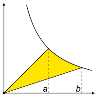
A hyperbolic sector is a region of the Cartesian plane bounded by a hyperbola and two rays from the origin to it. For example, the two points (a, 1/a) and (b, 1/b) on the rectangular hyperbola xy = 1, or the corresponding region when this hyperbola is re-scaled and its orientation is altered by a rotation leaving the center at the origin, as with the unit hyperbola. A hyperbolic sector in standard position has a = 1 and b > 1.
Hyperbolic sectors are the basis for the hyperbolic functions.
Area edit

The area of a hyperbolic sector in standard position is natural logarithm of b .
Proof: Integrate under 1/x from 1 to b, add triangle {(0, 0), (1, 0), (1, 1)}, and subtract triangle {(0, 0), (b, 0), (b, 1/b)} (both triangles of which have the same area). [1]
When in standard position, a hyperbolic sector corresponds to a positive hyperbolic angle at the origin, with the measure of the latter being defined as the area of the former.
Hyperbolic triangle edit

When in standard position, a hyperbolic sector determines a hyperbolic triangle, the right triangle with one vertex at the origin, base on the diagonal ray y = x, and third vertex on the hyperbola

with the hypotenuse being the segment from the origin to the point (x, y) on the hyperbola. The length of the base of this triangle is

and the altitude is

where u is the appropriate hyperbolic angle.
The analogy between circular and hyperbolic functions was described by Augustus De Morgan in his Trigonometry and Double Algebra (1849).[2] William Burnside used such triangles, projecting from a point on the hyperbola xy = 1 onto the main diagonal, in his article "Note on the addition theorem for hyperbolic functions".[3]
Hyperbolic logarithm edit

It is known that f(x) = xp has an algebraic antiderivative except in the case p = –1 corresponding to the quadrature of the hyperbola. The other cases are given by Cavalieri's quadrature formula. Whereas quadrature of the parabola had been accomplished by Archimedes in the third century BC (in The Quadrature of the Parabola), the hyperbolic quadrature required the invention in 1647 of a new function: Gregoire de Saint-Vincent addressed the problem of computing the areas bounded by a hyperbola. His findings led to the natural logarithm function, once called the hyperbolic logarithm since it is obtained by integrating, or finding the area, under the hyperbola.[4]
Before 1748 and the publication of Introduction to the Analysis of the Infinite, the natural logarithm was known in terms of the area of a hyperbolic sector. Leonhard Euler changed that when he introduced transcendental functions such as 10x. Euler identified e as the value of b producing a unit of area (under the hyperbola or in a hyperbolic sector in standard position). Then the natural logarithm could be recognized as the inverse function to the transcendental function ex.
To accommodate the case of negative logarithms and the corresponding negative hyperbolic angles, different hyperbolic sectors are constructed according to whether x is greater or less than one. A variable right triangle with area 1/2 is The isosceles case is The natural logarithm is known as the area under y = 1/x between one and x. A positive hyperbolic angle is given by the area of A negative hyperbolic angle is given by the negative of the area This convention is in accord with a negative natural logarithm for x in (0,1).


Hyperbolic geometry edit
When Felix Klein wrote his book on non-Euclidean geometry in 1928, he provided a foundation for the subject by reference to projective geometry. To establish hyperbolic measure on a line, he noted that the area of a hyperbolic sector provided visual illustration of the concept.[5]
Hyperbolic sectors can also be drawn to the hyperbola . The area of such hyperbolic sectors has been used to define hyperbolic distance in a geometry textbook.[6]

See also edit
References edit
- ^ V.G. Ashkinuse & Isaak Yaglom (1962) Ideas and Methods of Affine and Projective Geometry (in Russian), page 151, Ministry of Education, Moscow
- ^ Augustus De Morgan (1849) Trigonometry and Double Algebra, Chapter VI: "On the connection of common and hyperbolic trigonometry"
- ^ William Burnside (1890) Messenger of Mathematics 20:145–8, see diagram page 146
- ^ Martin Flashman The History of Logarithms from Humboldt State University
- ^ Felix Klein (1928) Vorlesungen über Nicht-Euklidische Geometrie, p. 173, figure 113, Julius Springer, Berlin
- ^ Jürgen Richter-Gebert (2011) Perspectives on Projective Geometry, p. 385, ISBN 9783642172854 MR2791970
- Mellen W. Haskell (1895) On the introduction of the notion of hyperbolic functions Bulletin of the American Mathematical Society 1(6):155–9.