


Summary
In physics and mathematics, the Ikeda map is a discrete-time dynamical system given by the complex map


The original map was proposed first by Kensuke Ikeda as a model of light going around across a nonlinear optical resonator (ring cavity containing a nonlinear[disambiguation needed] dielectric medium) in a more general form. It is reduced to the above simplified "normal" form by Ikeda, Daido and Akimoto [1][2] stands for the electric field inside the resonator at the n-th step of rotation in the resonator, and and are parameters which indicate laser light applied from the outside, and linear phase across the resonator, respectively. In particular the parameter is called dissipation parameter characterizing the loss of resonator, and in the limit of the Ikeda map becomes a conservative map.


The original Ikeda map is often used in another modified form in order to take the saturation effect of nonlinear dielectric medium into account:

A 2D real example of the above form is:


For , this system has a chaotic attractor.

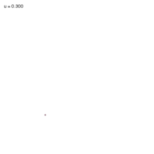
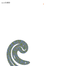
Attractor edit
This animation shows how the attractor of the system changes as the parameter is varied from 0.0 to 1.0 in steps of 0.01. The Ikeda dynamical system is simulated for 500 steps, starting from 20000 randomly placed starting points. The last 20 points of each trajectory are plotted to depict the attractor. Note the bifurcation of attractor points as is increased.

 |
 |
 |
 |


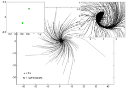
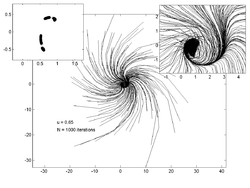
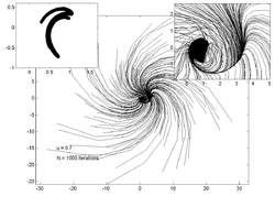
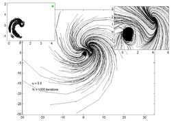
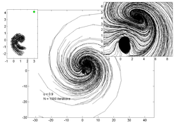
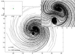
Point trajectories edit
The plots below show trajectories of 200 random points for various values of . The inset plot on the left shows an estimate of the attractor while the inset on the right shows a zoomed in view of the main trajectory plot.
 |
 |
 |
 |
 |
 |
 |
 |
 |
Octave/MATLAB code for point trajectories edit
The Octave/MATLAB code to generate these plots is given below:
% u = ikeda parameter
% option = what to plot
%  'trajectory' - plot trajectory of random starting points
%  'limit' - plot the last few iterations of random starting points
function ikeda(u, option)
P = 200; % how many starting points
N = 1000; % how many iterations
Nlimit = 20; % plot these many last points for 'limit' option

x = randn(1, P) * 10; % the random starting points
y = randn(1, P) * 10;

for n = 1:P,
    X = compute_ikeda_trajectory(u, x(n), y(n), N);

    switch option
        case 'trajectory' % plot the trajectories of a bunch of points
            plot_ikeda_trajectory(X); hold on;

        case 'limit'
            plot_limit(X, Nlimit); hold on;

        otherwise
            disp('Not implemented');
    end
end

axis tight; axis equal
text(- 25, - 15, ['u = ' num2str(u)]);
text(- 25, - 18, ['N = ' num2str(N) ' iterations']);
end

% Plot the last n points of the curve - to see end point or limit cycle
function plot_limit(X, n)
plot(X(end - n:end, 1), X(end - n:end, 2), 'ko');
end

% Plot the whole trajectory
function plot_ikeda_trajectory(X)
plot(X(:, 1), X(:, 2), 'k');
% hold on; plot(X(1,1), X(1,2), 'bo', 'markerfacecolor', 'g'); hold off
end

% u is the ikeda parameter
% x,y is the starting point
% N is the number of iterations
function [X] = compute_ikeda_trajectory(u, x, y, N)
X = zeros(N, 2);
X(1, :) = [x y];

for n = 2:N

    t = 0.4 - 6 / (1 + x ^ 2 + y ^ 2);
    x1 = 1 + u * (x * cos(t) - y * sin(t));
    y1 = u * (x * sin(t) + y * cos(t));
    x = x1;
    y = y1;

    X(n, :) = [x y];
end
end
Python code for point trajectories edit
import math

import matplotlib.pyplot as plt
import numpy as np

def main(u: float, points=200, iterations=1000, nlim=20, limit=False, title=True):
    """
    Args:
        u:float
            ikeda parameter
        points:int
            number of starting points
        iterations:int
            number of iterations
        nlim:int
            plot these many last points for 'limit' option. Will plot all points if set to zero
        limit:bool
            plot the last few iterations of random starting points if True. Else Plot trajectories.
        title:[str, NoneType]
            display the name of the plot if the value is affirmative
    """

    x = 10 * np.random.randn(points, 1)
    y = 10 * np.random.randn(points, 1)

    for n in range(points):
        X = compute_ikeda_trajectory(u, x[n][0], y[n][0], iterations)

        if limit:
            plot_limit(X, nlim)
            tx, ty = 2.5, -1.8

        else:
            plot_ikeda_trajectory(X)
            tx, ty = -30, -26

    plt.title(f"Ikeda Map ({u=:.2g}, {iterations=})") if title else None
    return plt

def compute_ikeda_trajectory(u: float, x: float, y: float, N: int):
    """Calculate a full trajectory

    Args:
        u - is the ikeda parameter
        x, y - coordinates of the starting point
        N - the number of iterations

    Returns:
        An array.
    """
    X = np.zeros((N, 2))

    for n in range(N):
        X[n] = np.array((x, y))

        t = 0.4 - 6 / (1 + x ** 2 + y ** 2)
        x1 = 1 + u * (x * math.cos(t) - y * math.sin(t))
        y1 = u * (x * math.sin(t) + y * math.cos(t))

        x = x1
        y = y1

    return X

def plot_limit(X, n: int) -> None:
    """
    Plot the last n points of the curve - to see end point or limit cycle

    Args:
        X: np.array
            trajectory of an associated starting-point
        n: int
            number of "last" points to plot
    """
    plt.plot(X[-n:, 0], X[-n:, 1], 'ko')

def plot_ikeda_trajectory(X) -> None:
    """
    Plot the whole trajectory

    Args:
        X: np.array
            trajectory of an associated starting-point
    """
    plt.plot(X[:,0], X[:, 1], "k")

if __name__ == "__main__":
    main(0.9, limit=True, nlim=0).show()
References edit
- ^ Ikeda, Kensuke (1979). "Multiple-valued stationary state and its instability of the transmitted light by a ring cavity system". Optics Communications. 30 (2). Elsevier BV: 257–261. Bibcode:1979OptCo..30..257I. CiteSeerX 10.1.1.158.7964. doi:10.1016/0030-4018(79)90090-7. ISSN 0030-4018.
- ^ Ikeda, K.; Daido, H.; Akimoto, O. (1980-09-01). "Optical Turbulence: Chaotic Behavior of Transmitted Light from a Ring Cavity". Physical Review Letters. 45 (9). American Physical Society (APS): 709–712. Bibcode:1980PhRvL..45..709I. doi:10.1103/physrevlett.45.709. ISSN 0031-9007.