


Summary
In celestial mechanics, a Kepler orbit (or Keplerian orbit, named after the German astronomer Johannes Kepler) is the motion of one body relative to another, as an ellipse, parabola, or hyperbola, which forms a two-dimensional orbital plane in three-dimensional space. A Kepler orbit can also form a straight line. It considers only the point-like gravitational attraction of two bodies, neglecting perturbations due to gravitational interactions with other objects, atmospheric drag, solar radiation pressure, a non-spherical central body, and so on. It is thus said to be a solution of a special case of the two-body problem, known as the Kepler problem. As a theory in classical mechanics, it also does not take into account the effects of general relativity. Keplerian orbits can be parametrized into six orbital elements in various ways.
In most applications, there is a large central body, the center of mass of which is assumed to be the center of mass of the entire system. By decomposition, the orbits of two objects of similar mass can be described as Kepler orbits around their common center of mass, their barycenter.
Introduction edit
From ancient times until the 16th and 17th centuries, the motions of the planets were believed to follow perfectly circular geocentric paths as taught by the ancient Greek philosophers Aristotle and Ptolemy. Variations in the motions of the planets were explained by smaller circular paths overlaid on the larger path (see epicycle). As measurements of the planets became increasingly accurate, revisions to the theory were proposed. In 1543, Nicolaus Copernicus published a heliocentric model of the Solar System, although he still believed that the planets traveled in perfectly circular paths centered on the Sun.[1]
Development of the laws edit
In 1601, Johannes Kepler acquired the extensive, meticulous observations of the planets made by Tycho Brahe. Kepler would spend the next five years trying to fit the observations of the planet Mars to various curves. In 1609, Kepler published the first two of his three laws of planetary motion. The first law states:
The orbit of every planet is an ellipse with the sun at a focus.
More generally, the path of an object undergoing Keplerian motion may also follow a parabola or a hyperbola, which, along with ellipses, belong to a group of curves known as conic sections. Mathematically, the distance between a central body and an orbiting body can be expressed as:

where:
- is the distance
- is the semi-major axis, which defines the size of the orbit
- is the eccentricity, which defines the shape of the orbit
- is the true anomaly, which is the angle between the current position of the orbiting object and the location in the orbit at which it is closest to the central body (called the periapsis).


Alternately, the equation can be expressed as:

Where is called the semi-latus rectum of the curve. This form of the equation is particularly useful when dealing with parabolic trajectories, for which the semi-major axis is infinite.

Despite developing these laws from observations, Kepler was never able to develop a theory to explain these motions.[2]
Isaac Newton edit
Between 1665 and 1666, Isaac Newton developed several concepts related to motion, gravitation and differential calculus. However, these concepts were not published until 1687 in the Principia, in which he outlined his laws of motion and his law of universal gravitation. His second of his three laws of motion states:
The acceleration of a body is parallel and directly proportional to the net force acting on the body, is in the direction of the net force, and is inversely proportional to the mass of the body:
Where:
- is the force vector
- is the mass of the body on which the force is acting
- is the acceleration vector, the second time derivative of the position vector


Strictly speaking, this form of the equation only applies to an object of constant mass, which holds true based on the simplifying assumptions made below.
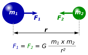
Newton's law of gravitation states:
Every point mass attracts every other point mass by a force pointing along the line intersecting both points. The force is proportional to the product of the two masses and inversely proportional to the square of the distance between the point masses:
where:
- is the magnitude of the gravitational force between the two point masses
- is the gravitational constant
- is the mass of the first point mass
- is the mass of the second point mass
- is the distance between the two point masses


From the laws of motion and the law of universal gravitation, Newton was able to derive Kepler's laws, which are specific to orbital motion in astronomy. Since Kepler's laws were well-supported by observation data, this consistency provided strong support of the validity of Newton's generalized theory, and unified celestial and ordinary mechanics. These laws of motion formed the basis of modern celestial mechanics until Albert Einstein introduced the concepts of special and general relativity in the early 20th century. For most applications, Keplerian motion approximates the motions of planets and satellites to relatively high degrees of accuracy and is used extensively in astronomy and astrodynamics.
Simplified two body problem edit
To solve for the motion of an object in a two body system, two simplifying assumptions can be made:
- The bodies are spherically symmetric and can be treated as point masses.
- There are no external or internal forces acting upon the bodies other than their mutual gravitation.
The shapes of large celestial bodies are close to spheres. By symmetry, the net gravitational force attracting a mass point towards a homogeneous sphere must be directed towards its centre. The shell theorem (also proven by Isaac Newton) states that the magnitude of this force is the same as if all mass was concentrated in the middle of the sphere, even if the density of the sphere varies with depth (as it does for most celestial bodies). From this immediately follows that the attraction between two homogeneous spheres is as if both had its mass concentrated to its center.
Smaller objects, like asteroids or spacecraft often have a shape strongly deviating from a sphere. But the gravitational forces produced by these irregularities are generally small compared to the gravity of the central body. The difference between an irregular shape and a perfect sphere also diminishes with distances, and most orbital distances are very large when compared with the diameter of a small orbiting body. Thus for some applications, shape irregularity can be neglected without significant impact on accuracy. This effect is quite noticeable for artificial Earth satellites, especially those in low orbits.
Planets rotate at varying rates and thus may take a slightly oblate shape because of the centrifugal force. With such an oblate shape, the gravitational attraction will deviate somewhat from that of a homogeneous sphere. At larger distances the effect of this oblateness becomes negligible. Planetary motions in the Solar System can be computed with sufficient precision if they are treated as point masses.
Two point mass objects with masses and and position vectors and relative to some inertial reference frame experience gravitational forces:


where is the relative position vector of mass 1 with respect to mass 2, expressed as:

and is the unit vector in that direction and is the length of that vector.

Dividing by their respective masses and subtracting the second equation from the first yields the equation of motion for the acceleration of the first object with respect to the second:
-
(1)

where is the gravitational parameter and is equal to


In many applications, a third simplifying assumption can be made:
- When compared to the central body, the mass of the orbiting body is insignificant. Mathematically, m1 >> m2, so α = G (m1 + m2) ≈ Gm1. Such standard gravitational parameters, often denoted as , are widely available for Sun, major planets and Moon, which have much larger masses than their orbiting satellites.


This assumption is not necessary to solve the simplified two body problem, but it simplifies calculations, particularly with Earth-orbiting satellites and planets orbiting the Sun. Even Jupiter's mass is less than the Sun's by a factor of 1047,[3] which would constitute an error of 0.096% in the value of α. Notable exceptions include the Earth-Moon system (mass ratio of 81.3), the Pluto-Charon system (mass ratio of 8.9) and binary star systems.
Under these assumptions the differential equation for the two body case can be completely solved mathematically and the resulting orbit which follows Kepler's laws of planetary motion is called a "Kepler orbit". The orbits of all planets are to high accuracy Kepler orbits around the Sun. The small deviations are due to the much weaker gravitational attractions between the planets, and in the case of Mercury, due to general relativity. The orbits of the artificial satellites around the Earth are, with a fair approximation, Kepler orbits with small perturbations due to the gravitational attraction of the Sun, the Moon and the oblateness of the Earth. In high accuracy applications for which the equation of motion must be integrated numerically with all gravitational and non-gravitational forces (such as solar radiation pressure and atmospheric drag) being taken into account, the Kepler orbit concepts are of paramount importance and heavily used.
Keplerian elements edit
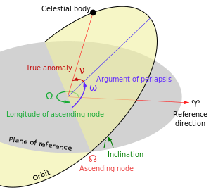
Any Keplerian trajectory can be defined by six parameters. The motion of an object moving in three-dimensional space is characterized by a position vector and a velocity vector. Each vector has three components, so the total number of values needed to define a trajectory through space is six. An orbit is generally defined by six elements (known as Keplerian elements) that can be computed from position and velocity, three of which have already been discussed. These elements are convenient in that of the six, five are unchanging for an unperturbed orbit (a stark contrast to two constantly changing vectors). The future location of an object within its orbit can be predicted and its new position and velocity can be easily obtained from the orbital elements.
Two define the size and shape of the trajectory:
- Semimajor axis ( )
- Eccentricity ( )
Three define the orientation of the orbital plane:
- Inclination ( ) defines the angle between the orbital plane and the reference plane.
- Longitude of the ascending node ( ) defines the angle between the reference direction and the upward crossing of the orbit on the reference plane (the ascending node).
- Argument of periapsis ( ) defines the angle between the ascending node and the periapsis.


And finally:
- True anomaly ( ) defines the position of the orbiting body along the trajectory, measured from periapsis. Several alternate values can be used instead of true anomaly, the most common being the mean anomaly and , the time since periapsis.


Because , and are simply angular measurements defining the orientation of the trajectory in the reference frame, they are not strictly necessary when discussing the motion of the object within the orbital plane. They have been mentioned here for completeness, but are not required for the proofs below.
Mathematical solution of the differential equation (1) above edit
For movement under any central force, i.e. a force parallel to r, the specific relative angular momentum stays constant:


Since the cross product of the position vector and its velocity stays constant, they must lie in the same plane, orthogonal to . This implies the vector function is a plane curve.

Because the equation has symmetry around its origin, it is easier to solve in polar coordinates. However, it is important to note that equation (1) refers to linear acceleration as opposed to angular or radial acceleration. Therefore, one must be cautious when transforming the equation. Introducing a cartesian coordinate system and polar unit vectors in the plane orthogonal to :


We can now rewrite the vector function and its derivatives as:

(see "Vector calculus"). Substituting these into (1), we find:

This gives the ordinary differential equation in the two variables and :
-
(2)

In order to solve this equation, all time derivatives must be eliminated. This brings:

-
(3)

Taking the time derivative of (3) gets
-
(4)

Equations (3) and (4) allow us to eliminate the time derivatives of . In order to eliminate the time derivatives of , the chain rule is used to find appropriate substitutions:
-
(5)

-
(6)

Using these four substitutions, all time derivatives in (2) can be eliminated, yielding an ordinary differential equation for as function of


-
(7)

The differential equation (7) can be solved analytically by the variable substitution
-
(8)

Using the chain rule for differentiation gets:
-
(9)

-
(10)

Using the expressions (10) and (9) for and gets


-
(11)

with the general solution
-
(12)

where e and are constants of integration depending on the initial values for s and


Instead of using the constant of integration explicitly one introduces the convention that the unit vectors defining the coordinate system in the orbital plane are selected such that takes the value zero and e is positive. This then means that is zero at the point where is maximal and therefore is minimal. Defining the parameter p as one has that


Alternate derivation edit
Another way to solve this equation without the use of polar differential equations is as follows:
Define a unit vector , , such that and . It follows that


Now consider
![{\displaystyle {\ddot {\mathbf {r} }}\times \mathbf {H} =-{\frac {\alpha }{r^{2}}}\mathbf {u} \times (r^{2}\mathbf {u} \times {\dot {\mathbf {u} }})=-\alpha \mathbf {u} \times (\mathbf {u} \times {\dot {\mathbf {u} }})=-\alpha [(\mathbf {u} \cdot {\dot {\mathbf {u} }})\mathbf {u} -(\mathbf {u} \cdot \mathbf {u} ){\dot {\mathbf {u} }}]}](https://wikimedia.org/api/rest_v1/media/math/render/svg/3af54235ba518c0147c3ffab79bb03a2fb35e68f)
(see Vector triple product). Notice that


Substituting these values into the previous equation gives:

Integrating both sides:

where c is a constant vector. Dotting this with r yields an interesting result:


Notice that are effectively the polar coordinates of the vector function. Making the substitutions and , we again arrive at the equation


-
(13)

This is the equation in polar coordinates for a conic section with origin in a focal point. The argument is called "true anomaly".
Eccentricity Vector edit
Notice also that, since is the angle between the position vector and the integration constant , the vector must be pointing in the direction of the periapsis of the orbit. We can then define the eccentricity vector associated with the orbit as:

where is the constant angular momentum vector of the orbit, and is the velocity vector associated with the position vector .


Obviously, the eccentricity vector, having the same direction as the integration constant , also points to the direction of the periapsis of the orbit, and it has the magnitude of orbital eccentricity. This makes it very useful in orbit determination (OD) for the orbital elements of an orbit when a state vector [ ] or [ ] is known.


Properties of trajectory equation edit
For this is a circle with radius p.

For this is an ellipse with

-
(14)

-
(15)

For this is a parabola with focal length


For this is a hyperbola with

-
(16)

-
(17)

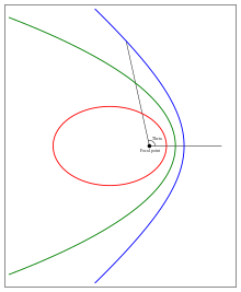
The following image illustrates a circle (grey), an ellipse (red), a parabola (green) and a hyperbola (blue)

The point on the horizontal line going out to the right from the focal point is the point with for which the distance to the focus takes the minimal value the pericentre. For the ellipse there is also an apocentre for which the distance to the focus takes the maximal value For the hyperbola the range for is


Using the chain rule for differentiation (5), the equation (2) and the definition of p as one gets that the radial velocity component is

-
(18)

and that the tangential component (velocity component perpendicular to ) is

-
(19)

The connection between the polar argument and time t is slightly different for elliptic and hyperbolic orbits.
For an elliptic orbit one switches to the "eccentric anomaly" E for which
-
(20)

-
(21)

and consequently
-
(22)

-
(23)

and the angular momentum H is
-
(24)

Integrating with respect to time t gives
-
(25)

under the assumption that time is selected such that the integration constant is zero.

As by definition of p one has
-
(26)

this can be written
-
(27)

For a hyperbolic orbit one uses the hyperbolic functions for the parameterisation
-
(28)

-
(29)

for which one has
-
(30)

-
(31)

and the angular momentum H is
-
(32)

Integrating with respect to time t gets
-
(33)

i.e.
-
(34)

To find what time t that corresponds to a certain true anomaly one computes corresponding parameter E connected to time with relation (27) for an elliptic and with relation (34) for a hyperbolic orbit.
Note that the relations (27) and (34) define a mapping between the ranges
![{\displaystyle \left[-\infty <t<\infty \right]\longleftrightarrow \left[-\infty <E<\infty \right]}](https://wikimedia.org/api/rest_v1/media/math/render/svg/40f4c2d85484a0f71543d4fe4ccd324f527a0142)
Some additional formulae edit
For an elliptic orbit one gets from (20) and (21) that
-
(35)

and therefore that
-
(36)

From (36) then follows that

From the geometrical construction defining the eccentric anomaly it is clear that the vectors and are on the same side of the x-axis. From this then follows that the vectors and are in the same quadrant. One therefore has that


-
(37)

and that
-
(38)

-
(39)

where " " is the polar argument of the vector and n is selected such that


For the numerical computation of the standard function ATAN2(y,x) (or in double precision DATAN2(y,x)) available in for example the programming language FORTRAN can be used.
Note that this is a mapping between the ranges
![{\displaystyle \left[-\infty <\theta <\infty \right]\longleftrightarrow \left[-\infty <E<\infty \right]}](https://wikimedia.org/api/rest_v1/media/math/render/svg/a733a34a4893dfafb8c3df87c470eeb8d9e324b9)
For a hyperbolic orbit one gets from (28) and (29) that
-
(40)

and therefore that
-
(41)

As


-
(42)

This relation is convenient for passing between "true anomaly" and the parameter E, the latter being connected to time through relation (34). Note that this is a mapping between the ranges
![{\displaystyle \left[-\cos ^{-1}\left(-{\frac {1}{e}}\right)<\theta <\cos ^{-1}\left(-{\frac {1}{e}}\right)\right]\longleftrightarrow \left[-\infty <E<\infty \right]}](https://wikimedia.org/api/rest_v1/media/math/render/svg/12031710e1f6bab0ee6c0d8d016315cd06e66813)


From relation (27) follows that the orbital period P for an elliptic orbit is
-
(43)

As the potential energy corresponding to the force field of relation (1) is


-
(44)

and from (13), (16), (18) and (19) that the sum of the kinetic and the potential energy for a hyperbolic orbit is
-
(45)

Relative the inertial coordinate system

-
(46)

-
(47)

The equation of the center relates mean anomaly to true anomaly for elliptical orbits, for small numerical eccentricity.
Determination of the Kepler orbit that corresponds to a given initial state edit
This is the "initial value problem" for the differential equation (1) which is a first order equation for the 6-dimensional "state vector" when written as

-
(48)

-
(49)

For any values for the initial "state vector" the Kepler orbit corresponding to the solution of this initial value problem can be found with the following algorithm:

Define the orthogonal unit vectors through

-
(50)

-
(51)

with and


From (13), (18) and (19) follows that by setting
-
(52)

and by defining and such that

-
(53)

-
(54)

where
-
(55)

one gets a Kepler orbit that for true anomaly has the same r, and values as those defined by (50) and (51).

If this Kepler orbit then also has the same vectors for this true anomaly as the ones defined by (50) and (51) the state vector of the Kepler orbit takes the desired values for true anomaly .
The standard inertially fixed coordinate system in the orbital plane (with directed from the centre of the homogeneous sphere to the pericentre) defining the orientation of the conical section (ellipse, parabola or hyperbola) can then be determined with the relation

-
(56)

-
(57)

Note that the relations (53) and (54) has a singularity when and


-
(58)

which is the case that it is a circular orbit that is fitting the initial state
The osculating Kepler orbit edit
For any state vector the Kepler orbit corresponding to this state can be computed with the algorithm defined above. First the parameters are determined from and then the orthogonal unit vectors in the orbital plane using the relations (56) and (57).


If now the equation of motion is
-
(59)

where


The Kepler orbit computed in this way having the same "state vector" as the solution to the "equation of motion" (59) at time t is said to be "osculating" at this time.
This concept is for example useful in case


is a small "perturbing force" due to for example a faint gravitational pull from other celestial bodies. The parameters of the osculating Kepler orbit will then only slowly change and the osculating Kepler orbit is a good approximation to the real orbit for a considerable time period before and after the time of osculation.
This concept can also be useful for a rocket during powered flight as it then tells which Kepler orbit the rocket would continue in case the thrust is switched off.
For a "close to circular" orbit the concept "eccentricity vector" defined as is useful. From (53), (54) and (56) follows that

-
(60)

i.e. is a smooth differentiable function of the state vector also if this state corresponds to a circular orbit.

See also edit
Citations edit
References edit
- El'Yasberg "Theory of flight of artificial earth satellites", Israel program for Scientific Translations (1967)
- Bate, Roger; Mueller, Donald; White, Jerry (1971). Fundamentals of Astrodynamics. Dover Publications, Inc., New York. ISBN 0-486-60061-0.
- Copernicus, Nicolaus (1952), "Book I, Chapter 4, The Movement of the Celestial Bodies Is Regular, Circular, and Everlasting-Or Else Compounded of Circular Movements", On the Revolutions of the Heavenly Spheres, Great Books of the Western World, vol. 16, translated by Charles Glenn Wallis, Chicago: William Benton, pp. 497–838
External links edit
- JAVA applet animating the orbit of a satellite in an elliptic Kepler orbit around the Earth with any value for semi-major axis and eccentricity.