


Summary
The Kuznets curve (/ˈkʌznɛts/) expresses a hypothesis advanced by economist Simon Kuznets in the 1950s and 1960s.[3] According to this hypothesis, as an economy develops, market forces first increase and then decrease economic inequality. The Kuznets curve appeared to be consistent with experience at the time it was proposed. However, since the 1970s, inequality has risen in the US and other developed countries, which invalidates the hypothesis.

Kuznets ratio and Kuznets curve edit
The Kuznets ratio is a measurement of the ratio of income going to the highest-earning households (usually defined by the upper 20%) to income going to the lowest-earning households,[4] which is commonly measured by either the lowest 20% or lowest 40% of income. Comparing 20% to 20%, a completely even distribution is expressed as 1; 20% to 40% changes this value to 0.5.
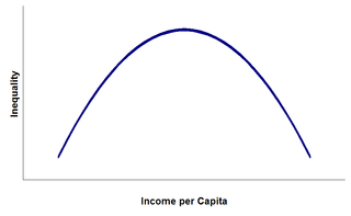
Kuznets curve diagrams show an inverted U curve, although variables along the axes are often mixed and matched, with inequality or the Gini coefficient on the Y axis and economic development, time or per-capita incomes on the X axis.[5]
Explanations edit
One explanation of such a progression suggests that early in development, investment opportunities for those who have money multiply, while an influx of cheap rural labor to the cities holds down wages. Whereas in mature economies, human capital accrual (an estimate of income that has been achieved but not yet consumed) takes the place of physical capital accrual as the main source of growth; and inequality slows growth by lowering education levels because poorer, disadvantaged people lack finance for their education in imperfect credit-markets.
The Kuznets curve implies that as a nation undergoes industrialization – and especially the mechanization of agriculture – the center of the nation's economy will shift to the cities. As internal migration by farmers looking for better-paying jobs in urban hubs causes a significant rural-urban inequality gap (the owners of firms would be profiting, while laborers from those industries would see their incomes rise at a much slower rate and agricultural workers would possibly see their incomes decrease), rural populations decrease as urban populations increase. Inequality is then expected to decrease when a certain level of average income is reached and the processes of industrialization – democratization and the rise of the welfare state – allow for the benefits from rapid growth, and increase the per-capita income. Kuznets believed that inequality would follow an inverted "U" shape as it rises and then falls again with the increase of income per-capita.[6] Kuznets had two similar explanations for this historical phenomenon:
- workers migrated from agriculture to industry; and
- rural workers moved to urban jobs.
In both explanations, inequality will decrease after 50% of the shift force switches over to the higher paying sector.[4]
Evidence edit
Inequality has risen in most developed countries since the 1960s, so that graphs of inequality over time no longer display a Kuznets curve. Piketty has argued that the decline in inequality over the first half of the 20th century was a once-off effect due to the destruction of large concentrations of wealth by war and economic depression.
The Kuznets curve and development economics edit
Critics of the Kuznets curve theory argue that its U-shape comes not from progression in the development of individual countries, but rather from historical differences between countries. For instance, many of the middle income countries used in Kuznets' data set were in Latin America, a region with historically high levels of inequality. When controlling for this variable, the U-shape of the curve tends to disappear (e.g. Deininger and Squire, 1998). Regarding the empirical evidence, based on large panels of countries or time series approaches, Fields (2001) considers the Kuznets hypothesis refuted.[7]
The East Asian miracle (EAM) has been used to criticize the validity of the Kuznets curve theory. The rapid economic growth of eight East Asian countries—Japan; the Four Asian Tigers South Korea, Taiwan, Singapore, Hong Kong; Indonesia, Thailand, and Malaysia—between 1965 and 1990, was called the East Asian miracle. The EAM defies the Kuznets curve, which insists growth produces inequality, and that inequality is a necessity for overall growth.[6][8] Manufacturing and export grew quickly and powerfully. Yet, contrary to Kuznets' historical examples, the EAM saw continual increases in life expectancy and decreasing rates of severe poverty.[9] Scholars have sought to understand how the EAM saw the benefits of rapid economic growth distributed broadly among the population.[8] Joseph Stiglitz explains this by the immediate re-investment of initial benefits into land reform (increasing rural productivity, income, and savings), universal education (providing greater equality and what Stiglitz calls an "intellectual infrastructure" for productivity[8]), and industrial policies that distributed income more equally through high and increasing wages and limited the price increases of commodities. These factors increased the average citizen's ability to consume and invest within the economy, further contributing to economic growth. Stiglitz highlights that the high rates of growth provided the resources to promote equality, which acted as a positive-feedback loop to support the high rates of growth.
Cambridge University Lecturer Gabriel Palma recently found no evidence for a 'Kuznets curve' in inequality:
"[T]he statistical evidence for the 'upwards' side of the 'Inverted-U' between inequality and income per capita seems to have vanished, as many low and low-middle income countries now have a distribution of income similar to that of most middle-income countries (other than those of Latin America and Southern Africa). That is, half of Sub-Saharan Africa and many countries in Asian, including India, China and Vietnam, now have an income distribution similar to that found in North Africa, the Caribbean and the second-tier NICs. And this level is also similar to that of half of the first-tier NICs, the Mediterranean EU and the Anglophone OECD (excluding the US). As a result, about 80% of the world population now live in countries with a Gini around 40."[10]
Palma goes on to note that, among middle-income countries, only those in Latin America and Southern Africa live in an inequality league of their own. Instead of a Kuznets curve, he breaks the population into deciles and examines the relationship between their respective incomes and income inequality. Palma then shows that there are two distributional trends taking place in inequality within a country:
"One is 'centrifugal', and takes place at the two tails of the distribution—leading to an increased diversity across countries in the shares appropriated by the top 10 percent and bottom forty percent. The other is 'centripetal', and takes place in the middle—leading to a remarkable uniformity across countries in the share of income going to the half of the population located between deciles 5 to 9."[10]
Therefore, it is the share of the richest 10% of the population that affects the share of the poorest 40% of the population with the middle to upper-middle staying the same across all countries.
In Capital in the Twenty-First Century, Thomas Piketty denies the effectiveness of the Kuznets curve. He points out that in some rich countries, the level of income inequality in 21st century has exceeded that in the second decades of 20th century, proposing the explanation that when the rate of return on capital is greater than the rate of economic growth over the long term, the result is the concentration of wealth.[11]
Kuznets's own caveats edit
In a biography about Simon Kuznets's scientific methods, economist Robert Fogel noted Kuznets's own reservations about the "fragility of the data" which underpinned the hypothesis. Fogel notes that most of Kuznets's paper was devoted to explicating the conflicting factors at play. Fogel emphasized Kuznets's opinion that "even if the data turned out to be valid, they pertained to an extremely limited period of time and to exceptional historical experiences." Fogel noted that despite these "repeated warnings", Kuznets's caveats were overlooked, and the Kuznets curve was "raised to the level of law" by other economists.[12]
Inequality and trade liberalization edit
Dobson and Ramlogan's research looked to identify the relationship between inequality and trade liberalization. There have been mixed findings with this idea – some developing countries have experienced greater inequality, less inequality, or no difference at all, due to trade liberalization. Because of this, Dobson and Ramlogan suggest that perhaps trade openness can be related to inequality through a Kuznets curve framework.[13] A trade liberalization-versus-inequality graph measures trade openness along the x-axis and inequality along the y-axis. Dobson and Ramlogan determine trade openness by the ratio of exports and imports (the total trade) and the average tariff rate; inequality is determined by gross primary school enrolment rates, the share of agriculture in total output, the rate of inflation, and cumulative privatization.[13] By studying data from several Latin American countries that have implemented trade liberalization policies in the past 30 years, the Kuznets curve seems to apply to the relationship between trade liberalization and inequality (measured by the GINI coefficient).[13] However, many of these nations saw a shift from low-skill labour production to natural resource intensive activities. This shift would not benefit low-skill workers as much. So although their evidence seems to support the Kuznets theory in relation to trade liberalization, Dobson and Ramlogan assert that policies for redistribution must be simultaneously implemented in order to mitigate the initial increase in inequality.[13]
Environmental Kuznets curve edit

The environmental Kuznets curve (EKC) is a hypothesized relationship between environmental quality and economic development:[14] various indicators of environmental degradation tend to get worse as modern economic growth occurs until average income reaches a certain point over the course of development.[15][16] The EKC suggests, in sum, that "the solution to pollution is economic growth."
Although subject to continuing debate, there is considerable evidence to support the application of environmental Kuznets curve for various environmental health indicators, such as water, air pollution and ecological footprint which show the inverted U-shaped curve as per capita income and/or GDP rise.[17][18] It has been argued that this trend occurs in the level of many of the environmental pollutants, such as sulfur dioxide, nitrogen oxide, lead, DDT, chlorofluorocarbons, sewage, and other chemicals previously released directly into the air or water. For example, between 1970 and 2006, the United States' inflation-adjusted GDP grew by 195%, the number of cars and trucks in the country more than doubled, and the total number of miles driven increased by 178%. However, during that same period certain regulatory changes and technological innovations led to decreases in annual emissions of carbon monoxide from 197 million tons to 89 million, nitrogen oxides emissions from 27 million tons to 19 million, sulfur dioxide emissions from 31 million tons to 15 million, particulate emissions by 80%, and lead emissions by more than 98%.[19]
Deforestation may follow a Kuznets curve (cf. forest transition curve). Among countries with a per capita GDP of at least $4,600, net deforestation has ceased.[20] Yet it has been argued that wealthier countries are able to maintain forests along with high consumption by 'exporting' deforestation, leading to continuing deforestation on a worldwide scale.[21]
Criticisms edit
However, the EKC model is debatable when applied to other pollutants, some natural resource use, and biodiversity conservation.[22] For example, energy, land and resource use (sometimes called the "ecological footprint") may not fall with rising income.[23] While the ratio of energy per real GDP has fallen, total energy use is still rising in most developed countries as are total emission of many greenhouse gases. Additionally, the status of many key "ecosystem services" provided by ecosystems, such as freshwater provision (Perman, et al., 2003), soil fertility,[citation needed] and fisheries,[citation needed] have continued to decline in developed countries. Proponents of the EKC argue that this varied relationship does not necessarily invalidate the hypothesis, but instead that the applicability of the Kuznets curves to various environmental indicators may differ when considering different ecosystems, economics, regulatory schemes, and technologies.
At least one critic argues that the US is still struggling to attain the income level necessary to prioritize certain environmental pollutants such as carbon emissions, which have yet to follow the EKC.[24] Yandle et al. argue that the EKC has not been found to apply to carbon because most pollutants create localized problems like lead and sulfur, so there are a greater urgency and response to cleaning up such pollutants. As a country develops, the marginal value of cleaning up such pollutants makes a large direct improvement to the quality of citizens' lives. Conversely, reducing carbon dioxide emissions does not have a dramatic impact at a local level, so the impetus to clean them up is only for the altruistic reason of improving the global environment. This becomes a tragedy of the commons where it is most efficient for everyone to pollute and for no one to clean up, and everyone is worse as a result (Hardin, 1968). Thus, even in a country like the US with a high level of income, carbon emissions are not decreasing in accordance with the EKC.[24] However, there seems to be little consensus about whether EKC is formed with regard to CO2 emissions, as CO2 is a global pollutant that has yet to prove its validity within Kuznet's Curve.[25] That said, Yandle et al. also concluded that "policies that stimulate growth (trade liberalization, economic restructuring, and price reform) should be good for the environment".[24]
Other critics point out that researchers also disagree about the shape of the curve when longer-term time scales are evaluated. For example, Millimet and Stengos regard the traditional "inverse U" shape as actually being an "N" shape, indicating that pollution increases as a country develops, decreases once the threshold GDP is reached, and then begins increasing as national income continues to increase. While such findings are still being debated, it could prove to be important because it poses the concerning question of whether pollution actually begins to decline for good when an economic threshold is reached or whether the decrease is only in local pollutants and pollution is simply exported to poorer developing countries. Levinson concludes that the environmental Kuznets curve is insufficient to support a pollution policy regardless whether it is laissez-faire or interventionist, although the literature has been used this way by the press.[26]
Arrow et al. argue pollution-income progression of agrarian communities (clean) to industrial economies (pollution intensive) to service economies (cleaner) would appear to be false if pollution increases again at the end due to higher levels of income and consumption of the population at large.[27] A difficulty with this model is that it lacks predictive power because it is highly uncertain how the next phase of economic development will be characterized. [citation needed]
Suri and Chapman argue that the EKC is not applicable on the global scale, as a net pollution reduction may not actually be occurring globally. Wealthy nations have a trend of exporting the activities that create the most pollution, like manufacturing of clothing and furniture, to poorer nations that are still in the process of industrial development (Suri and Chapman, 1998). This could mean that as the world's poor nations develop, they will have nowhere to export their pollution. Thus, this progression of environmental clean-up occurring in conjunction with economic growth cannot be replicated indefinitely because there may be nowhere to export waste and pollution-intensive processes. However, Gene Grossman and Alan B. Krueger, the authors who initially made the correlation between economic growth, environmental clean-up, and the Kuznets curve, conclude that there is "no evidence that environmental quality deteriorates steadily with economic growth."[26]
Stern warns "it is very easy to do bad econometrics", and says "the history of the EKC exemplifies what can go wrong". He finds that "little or no attention has been paid to the statistical properties of the data used such as serial dependence or stochastic trends in time series and few tests of model adequacy have been carried out or presented. However, one of the main purposes of doing econometrics is to test which apparent relationships ... are valid and which are spurious correlations". He states his unequivocal finding: "When we do take such statistics into account and use appropriate techniques we find that the EKC does not exist (Perman and Stern 2003). Instead, we get a more realistic view of the effect of economic growth and technological changes on environmental quality. It seems that most indicators of environmental degradation are monotonically rising in income though the 'income elasticity' is less than one and is not a simple function of income alone. Time-related effects reduce environmental impacts in countries at all levels of income. However, in rapidly growing middle income countries the scale effect, which increases pollution and other degradation, overwhelms the time effect. For example, Armenia, after gaining its independence from the Soviet Union, has become the country with the least income elasticity in Eastern Europe and Central Asia.[28] In wealthy countries, growth is slower, and pollution reduction efforts can overcome the scale effect. This is the origin of the apparent EKC effect".[29]
Kuznets curves for steel and other metals edit
Steel production has been shown to follow a Kuznets-type curve in the national development cycles of a range of economies, including the United States, Japan, Republic of Korea and China. This discovery, and the first usage of the term "Kuznets Curve for Steel" and "Metal intensity Kuznets Curve" were by Huw McKay in a 2008 working paper (McKay 2008). This was subsequently developed in McKay (2012). A body of work on "Material Kuznets Curves" focused on non-ferrous metals has also emerged as academic and policy interest in resource intensity increased during the first two decades of the 21st century.[citation needed]
References edit
- ^ Based on Table TI.1 of the supplement Archived 8 May 2014 at the Wayback Machine to Thomas Piketty's Capital in the Twenty-First Century.
- ^ Piketty, Thomas (2013). Capital in the Twenty-First Century. Belknap. p. 24.
- ^ Kuznets profileArchived 18 September 2009 at the Wayback Machine at New School for Social Research: "...his discovery of the inverted U-shaped relation between income inequality and economic growth..."
- ^ a b Kuznets, Simon. 1955. Economic Growth and Income Inequality. American Economic Review 45 (March): 1–28.
- ^ Vuong, Q.-H.; Ho, M.-T.; Nguyen, T. H.-K.; Nguyen, M.-H. (2019). "The trilemma of sustainable industrial growth: evidence from a piloting OECD's Green city". Palgrave Communications. 5: 156. doi:10.1057/s41599-019-0369-8.
- ^ a b Galbraith, James (2007). "Global inequality and global macroeconomics". Journal of Policy Modeling. 29 (4): 587–607. CiteSeerX 10.1.1.454.8135. doi:10.1016/j.jpolmod.2007.05.008.
- ^ Fields G (2001). Distribution and Development, A New Look at the Developing World. Russel Sage Foundation, New York, and The MIT Press, Cambridge, Massachusetts, and London.
- ^ a b c Stiglitz, Joseph E. (August 1996). "Some Lessons From The East Asian Miracle". The World Bank Research Observer. 11 (2): 151–177. CiteSeerX 10.1.1.1017.9460. doi:10.1093/wbro/11.2.151.
- ^ (course lectures).
- ^ a b Palma, J. G. (26 January 2011). "Homogeneous middles vs. heterogeneous tails, and the end of the 'Inverted-U': the share of the rich is what it's all about". Cambridge Working Papers in Economics.
- ^ Thomas Piketty (2014). Capital in the Twenty-First Century. Belknap Press. ISBN 978-0674430006.
- ^ Fogel, Robert W. (December 1987). Some Notes on the Scientific Methods of Simon Kuznets. National Bureau of Economic Research. pp. 26–7. doi:10.3386/w2461. S2CID 142683345.
- ^ a b c d Dobson, Stephen; Carlyn Ramlogan (April 2009). "Is There An Openness Kuznets Curve?". Kyklos. 62 (2): 226–238. doi:10.1111/j.1467-6435.2009.00433.x. S2CID 154528726.
- ^ Yasin, Iftikhar; Ahmad, Nawaz; Chaudhary, Muhammad Aslam (22 July 2020). "The impact of financial development, political institutions, and urbanization on environmental degradation: evidence from 59 less-developed economies". Environment, Development and Sustainability. 23 (5): 6698–6721. doi:10.1007/s10668-020-00885-w. ISSN 1573-2975. S2CID 220721520.
- ^ Shafik, Nemat. 1994. Economic development and environmental quality: an econometric analysis. Oxford Economic Papers 46 (October): 757–773
- ^ Grossman, G. M.; Krueger, A. B. (1991). "Environmental impacts of a North American Free Trade Agreement". National Bureau of Economic Research Working Paper 3914, NBER. doi:10.3386/w3914.
- ^ Yasin, Iftikhar; Ahmad, Nawaz; Chaudhary, M. Aslam (22 July 2019). "Catechizing the Environmental-Impression of Urbanization, Financial Development, and Political Institutions: A Circumstance of Ecological Footprints in 110 Developed and Less-Developed Countries". Social Indicators Research. 147 (2): 621–649. doi:10.1007/s11205-019-02163-3. ISSN 0303-8300. S2CID 199855869.
- ^ John Tierney (20 April 2009). "The Richer-Is-Greener Curve". The New York Times.
- ^ "Don't Be Very Worried". The Wall St. Journal. 23 May 2006. Archived from the original on 15 June 2006.
{{cite news}}: CS1 maint: bot: original URL status unknown (link) - ^ Returning forests analyzed with the forest identity, 2006, by Pekka E. Kauppi (Department of Biological and Environmental Sciences, University of Helsinki), Jesse H. Ausubel (Program for the Human Environment, The Rockefeller University), Jingyun Fang (Department of Ecology, Peking University), Alexander S. Mather (Department of Geography and Environment, University of Aberdeen), Roger A. Sedjo (Resources for the Future), and Paul E. Waggoner (Connecticut Agricultural Experiment Station)
- ^ "Developing countries often outsource deforestation, study finds". Stanford News. 24 November 2010. Retrieved 18 June 2015.
- ^ Mills JH, Waite TA (2009). "Economic prosperity, biodiversity conservation, and the environmental Kuznets curve". Ecological Economics. 68 (7): 2087–2095. doi:10.1016/j.ecolecon.2009.01.017.
- ^ "Google Public Data US Energy". Energy Information Administration. Retrieved 17 December 2011.
- ^ a b c Yandle B, Vijayaraghavan M, Bhattarai M (2002). "The Environmental Kuznets Curve: A Primer". The Property and Environment Research Center. Archived from the original on 30 December 2008. Retrieved 16 June 2008.
- ^ Uchiyama, Katsuhisa (2016). Environmental Kuznets Curve Hypothesis and Carbon Dioxide Emissions - Springer. SpringerBriefs in Economics. doi:10.1007/978-4-431-55921-4. ISBN 978-4-431-55919-1.
- ^ a b Arik Levinson (2000). The Ups and Downs of the Environmental Kuznets Curve. Georgetown University. CiteSeerX 10.1.1.92.2062.
- ^ Arrow K, Bolin B, Costanza R, Dasgupta P, Folke C, Holling CS, et al. (1995). "Economic growth, carrying capacity, and the environment". Ecological Economics. 15 (2): 91–95. doi:10.1016/0921-8009(95)00059-3. PMID 17756719.
- ^ Koilo, Viktoriia. 2019. "Evidence of the Environmental Kuznets Curve: Unleashing the Opportunity of Industry 4.0 in Emerging Economies" Journal of Risk and Financial Management 12, no. 3: 122. https://doi.org/10.3390/jrfm12030122
- ^ David I. Stern. "The Environmental Kuznets Curve" (PDF). International Society for Ecological Economics Internet Encyclopedia of Ecological Economics. Archived from the original (PDF) on 20 July 2011. Retrieved 17 March 2019.
Bibliography edit
- Brenner, Y.S., Hartmut Kaelble, and Mark Thomas (1991): Income Distribution in Historical Perspective. Cambridge University Press.
- Deininger K, Squire L (1998). "New Ways of Looking at Old Issues: Inequality and Growth". Journal of Development Economics. 57 (2): 259–287. doi:10.1016/s0304-3878(98)00099-6.
- Fields G (2001). Distribution and Development, A New Look at the Developing World. Russel Sage Foundation, New York, and The MIT Press, Cambridge, Massachusetts, and London.
- Palma, JG (2011). "Homogeneous middles vs. heterogeneous tails, and the end of the 'Inverted-U': it's all about the share of the rich". Development and Change. 42: 87–153. doi:10.1111/j.1467-7660.2011.01694.x.
- McKay, Huw (2008) ‘Metal intensity in comparative historical perspective: China, North Asia, the United States and the Kuznets curve’, Global Dynamic Systems Centre working papers, no. 6, September.
- McKay, Huw (2012) ‘Metal intensity in comparative historical perspective: China, North Asia, the United States ’, chapter 2 in Ligang Song and Haimin Lu (eds) The Chinese Steel Industry’s Transformation: Structural Change, Performance and Demand on Resources, Edward Elgar: Cheltenham UK.
- Van Zanden, J. L. (1995). "Tracing the Beginning of the Kuznets Curve: Western Europe during the Early Modern Period". The Economic History Review. 48 (4): 643–664. doi:10.2307/2598128. JSTOR 2598128.