


Summary
In probability theory, a log-normal (or lognormal) distribution is a continuous probability distribution of a random variable whose logarithm is normally distributed. Thus, if the random variable X is log-normally distributed, then Y = ln(X) has a normal distribution.[2][3] Equivalently, if Y has a normal distribution, then the exponential function of Y, X = exp(Y) , has a log-normal distribution. A random variable which is log-normally distributed takes only positive real values. It is a convenient and useful model for measurements in exact and engineering sciences, as well as medicine, economics and other topics (e.g., energies, concentrations, lengths, prices of financial instruments, and other metrics).
|
Probability density function  Identical parameter but differing parameters | |||
|
Cumulative distribution function  | |||
| Notation | |||
|---|---|---|---|
| Parameters |
(logarithm of scale), | ||
| Support | |||
| CDF | |||
| Quantile | |||
| Mean | |||
| Median | |||
| Mode | |||
| Variance | |||
| Skewness | |||
| Excess kurtosis | |||
| Entropy | |||
| MGF |
defined only for numbers with a non-positive real part, see text | ||
| CF |
representation is asymptotically divergent, but adequate for most numerical purposes | ||
| Fisher information | |||
| Method of Moments |
| ||
| Expected shortfall | [1] | ||


![{\displaystyle \ {\frac {\ 1\ }{2}}\left[1+\operatorname {erf} \left({\frac {\ \ln x-\mu \ }{\sigma {\sqrt {2\ }}}}\right)\right]=\Phi \left({\frac {\ln(x)-\mu }{\sigma }}\right)}](https://wikimedia.org/api/rest_v1/media/math/render/svg/8c51991c6608ba25efced3e0a4107e57c9b0c42d)


![{\displaystyle \ \left[\ \exp(\sigma ^{2})-1\ \right]\ \exp \left(2\ \mu +\sigma ^{2}\right)\ }](https://wikimedia.org/api/rest_v1/media/math/render/svg/32a3c017965f320e31686d9dca9506e857b83166)
![{\displaystyle \ \left[\ \exp \left(\sigma ^{2}\right)+2\ \right]{\sqrt {\exp(\sigma ^{2})-1\;}}}](https://wikimedia.org/api/rest_v1/media/math/render/svg/1657430133ee87501a9b184a9f8cd9f01d00fa12)


![{\displaystyle \ \mu =\log \left({\frac {\operatorname {\mathbb {E} } [X]\ }{\ {\sqrt {{\frac {\ \operatorname {Var} [X]~~}{\ \operatorname {\mathbb {E} } [X]^{2}\ }}+1\ }}\ }}\right)\ ,}](https://wikimedia.org/api/rest_v1/media/math/render/svg/55074cffa7b5b5f102b010be57837a25279bf580)
![{\displaystyle \ \sigma ={\sqrt {\log \left({\frac {\ \operatorname {Var} [X]~~}{\ \operatorname {\mathbb {E} } [X]^{2}\ }}+1\ \right)\ }}}](https://wikimedia.org/api/rest_v1/media/math/render/svg/46349b67d9ab6239b10e582d5c92ad410254a97e)

The distribution is occasionally referred to as the Galton distribution or Galton's distribution, after Francis Galton.[4] The log-normal distribution has also been associated with other names, such as McAlister, Gibrat and Cobb–Douglas.[4]
A log-normal process is the statistical realization of the multiplicative product of many independent random variables, each of which is positive. This is justified by considering the central limit theorem in the log domain (sometimes called Gibrat's law). The log-normal distribution is the maximum entropy probability distribution for a random variate X—for which the mean and variance of ln(X) are specified.[5]
Definitions edit
Generation and parameters edit
Let be a standard normal variable, and let and be two real numbers, with . Then, the distribution of the random variable


is called the log-normal distribution with parameters and . These are the expected value (or mean) and standard deviation of the variable's natural logarithm, not the expectation and standard deviation of itself.


This relationship is true regardless of the base of the logarithmic or exponential function: If is normally distributed, then so is for any two positive numbers Likewise, if is log-normally distributed, then so is where .


In order to produce a distribution with desired mean and variance one uses and


Alternatively, the "multiplicative" or "geometric" parameters and can be used. They have a more direct interpretation: is the median of the distribution, and is useful for determining "scatter" intervals, see below.


Probability density function edit
A positive random variable is log-normally distributed (i.e., ), if the natural logarithm of is normally distributed with mean and variance


Let and be respectively the cumulative probability distribution function and the probability density function of the standard normal distribution, then we have that[2][4] the probability density function of the log-normal distribution is given by:


![{\displaystyle {\begin{aligned}f_{X}(x)&={\frac {\rm {d}}{{\rm {d}}x}}\ \operatorname {\mathbb {P} _{\mathit {X}}} \,\!{\bigl [}\ X\leq x\ {\bigr ]}\\[6pt]&={\frac {\rm {d}}{{\rm {d}}x}}\ \operatorname {\mathbb {P} _{\mathit {X}}} \,\!{\bigl [}\ \ln X\leq \ln x\ {\bigr ]}\\[6pt]&={\frac {\rm {d}}{{\rm {d}}x}}\operatorname {\Phi } \!\!\left({\frac {\ \ln x-\mu \ }{\sigma }}\right)\\[6pt]&=\operatorname {\varphi } \!\left({\frac {\ln x-\mu }{\sigma }}\right){\frac {\rm {d}}{{\rm {d}}x}}\left({\frac {\ \ln x-\mu \ }{\sigma }}\right)\\[6pt]&=\operatorname {\varphi } \!\left({\frac {\ \ln x-\mu \ }{\sigma }}\right){\frac {1}{\ \sigma \ x\ }}\\[6pt]&={\frac {1}{\ x\ \sigma {\sqrt {2\ \pi \ }}\ }}\exp \left(-{\frac {\ (\ln x-\mu )^{2}\ }{2\ \sigma ^{2}}}\right)~.\end{aligned}}}](https://wikimedia.org/api/rest_v1/media/math/render/svg/c10dc2a3d559ddc86174a24365d121314f6131cf)
Cumulative distribution function edit
The cumulative distribution function is

where is the cumulative distribution function of the standard normal distribution (i.e., ).

This may also be expressed as follows:[2]
![{\displaystyle {\frac {1}{2}}\left[1+\operatorname {erf} \left({\frac {\ln x-\mu }{\sigma {\sqrt {2}}}}\right)\right]={\frac {1}{2}}\operatorname {erfc} \left(-{\frac {\ln x-\mu }{\sigma {\sqrt {2}}}}\right)}](https://wikimedia.org/api/rest_v1/media/math/render/svg/d7373f66d2a24f5817a8bc2f2f44836941b79118)
where erfc is the complementary error function.
Multivariate log-normal edit
If is a multivariate normal distribution, then has a multivariate log-normal distribution.[6][7] The exponential is applied elementwise to the random vector . The mean of is


![{\displaystyle \operatorname {E} [{\boldsymbol {Y}}]_{i}=e^{\mu _{i}+{\frac {1}{2}}\Sigma _{ii}},}](https://wikimedia.org/api/rest_v1/media/math/render/svg/488f8b7b6e5331b3d4b257c87b40752a01ee6293)
and its covariance matrix is
![{\displaystyle \operatorname {Var} [{\boldsymbol {Y}}]_{ij}=e^{\mu _{i}+\mu _{j}+{\frac {1}{2}}(\Sigma _{ii}+\Sigma _{jj})}(e^{\Sigma _{ij}}-1).}](https://wikimedia.org/api/rest_v1/media/math/render/svg/11b3d9175a3f442f40eb4687f58014c3efdfa7d0)
Since the multivariate log-normal distribution is not widely used, the rest of this entry only deals with the univariate distribution.
Characteristic function and moment generating function edit
All moments of the log-normal distribution exist and
![{\displaystyle \operatorname {E} [X^{n}]=e^{n\mu +n^{2}\sigma ^{2}/2}}](https://wikimedia.org/api/rest_v1/media/math/render/svg/1ec49bbb5852b6e735f0a6a49468771db326b7bf)
This can be derived by letting within the integral. However, the log-normal distribution is not determined by its moments.[8] This implies that it cannot have a defined moment generating function in a neighborhood of zero.[9] Indeed, the expected value is not defined for any positive value of the argument , since the defining integral diverges.

![{\displaystyle \operatorname {E} [e^{tX}]}](https://wikimedia.org/api/rest_v1/media/math/render/svg/0379eb85a8f71d1d2e06107ba42758bc26c355b6)

The characteristic function is defined for real values of t, but is not defined for any complex value of t that has a negative imaginary part, and hence the characteristic function is not analytic at the origin. Consequently, the characteristic function of the log-normal distribution cannot be represented as an infinite convergent series.[10] In particular, its Taylor formal series diverges:
![{\displaystyle \operatorname {E} [e^{itX}]}](https://wikimedia.org/api/rest_v1/media/math/render/svg/33bdf53bdb972f0154a057c687c9545db5e7ff7d)

However, a number of alternative divergent series representations have been obtained.[10][11][12][13]
A closed-form formula for the characteristic function with in the domain of convergence is not known. A relatively simple approximating formula is available in closed form, and is given by[14]


where is the Lambert W function. This approximation is derived via an asymptotic method, but it stays sharp all over the domain of convergence of .


Properties edit


Probability in different domains edit
The probability content of a log-normal distribution in any arbitrary domain can be computed to desired precision by first transforming the variable to normal, then numerically integrating using the ray-trace method.[15] (Matlab code)
Probabilities of functions of a log-normal variable edit
Since the probability of a log-normal can be computed in any domain, this means that the cdf (and consequently pdf and inverse cdf) of any function of a log-normal variable can also be computed.[15] (Matlab code)
Geometric or multiplicative moments edit
The geometric or multiplicative mean of the log-normal distribution is . It equals the median. The geometric or multiplicative standard deviation is .[16][17]
![{\displaystyle \operatorname {GM} [X]=e^{\mu }=\mu ^{*}}](https://wikimedia.org/api/rest_v1/media/math/render/svg/9445c2ca179a4932cdadf4b511c0348c3449a4ea)
![{\displaystyle \operatorname {GSD} [X]=e^{\sigma }=\sigma ^{*}}](https://wikimedia.org/api/rest_v1/media/math/render/svg/1d39b3e467b86b861d3c19285f10f6d7dc8ec923)
By analogy with the arithmetic statistics, one can define a geometric variance, , and a geometric coefficient of variation,[16] , has been proposed. This term was intended to be analogous to the coefficient of variation, for describing multiplicative variation in log-normal data, but this definition of GCV has no theoretical basis as an estimate of itself (see also Coefficient of variation).
![{\displaystyle \operatorname {GVar} [X]=e^{\sigma ^{2}}}](https://wikimedia.org/api/rest_v1/media/math/render/svg/3a8446c1bc836c47f03e578df8e5971015871417)
![{\displaystyle \operatorname {GCV} [X]=e^{\sigma }-1}](https://wikimedia.org/api/rest_v1/media/math/render/svg/521d8430003df46e507169d1e2fd3ee976b4105e)

Note that the geometric mean is smaller than the arithmetic mean. This is due to the AM–GM inequality and is a consequence of the logarithm being a concave function. In fact,
![{\displaystyle \operatorname {E} [X]=e^{\mu +{\frac {1}{2}}\sigma ^{2}}=e^{\mu }\cdot {\sqrt {e^{\sigma ^{2}}}}=\operatorname {GM} [X]\cdot {\sqrt {\operatorname {GVar} [X]}}.}](https://wikimedia.org/api/rest_v1/media/math/render/svg/e16c0e50545da50c815d65794d7589b9bf513be4)
In finance, the term is sometimes interpreted as a convexity correction. From the point of view of stochastic calculus, this is the same correction term as in Itō's lemma for geometric Brownian motion.

Arithmetic moments edit
For any real or complex number n, the n-th moment of a log-normally distributed variable X is given by[4]
![{\displaystyle \operatorname {E} [X^{n}]=e^{n\mu +{\frac {1}{2}}n^{2}\sigma ^{2}}.}](https://wikimedia.org/api/rest_v1/media/math/render/svg/a4b6efe7347f26a8054654edcdfb03eb8b28bbf1)
Specifically, the arithmetic mean, expected square, arithmetic variance, and arithmetic standard deviation of a log-normally distributed variable X are respectively given by:[2]
![{\displaystyle {\begin{aligned}\operatorname {E} [X]&=e^{\mu +{\tfrac {1}{2}}\sigma ^{2}},\\[4pt]\operatorname {E} [X^{2}]&=e^{2\mu +2\sigma ^{2}},\\[4pt]\operatorname {Var} [X]&=\operatorname {E} [X^{2}]-\operatorname {E} [X]^{2}=(\operatorname {E} [X])^{2}(e^{\sigma ^{2}}-1)=e^{2\mu +\sigma ^{2}}(e^{\sigma ^{2}}-1),\\[4pt]\operatorname {SD} [X]&={\sqrt {\operatorname {Var} [X]}}=\operatorname {E} [X]{\sqrt {e^{\sigma ^{2}}-1}}=e^{\mu +{\tfrac {1}{2}}\sigma ^{2}}{\sqrt {e^{\sigma ^{2}}-1}},\end{aligned}}}](https://wikimedia.org/api/rest_v1/media/math/render/svg/2b59e2bead4a03f70fcf34a610106ae8704959a6)
The arithmetic coefficient of variation is the ratio . For a log-normal distribution it is equal to[3]
![{\displaystyle \operatorname {CV} [X]}](https://wikimedia.org/api/rest_v1/media/math/render/svg/89fe40c7a2788b7bb2797aeda4b90c1f53be8ce0)
![{\displaystyle {\tfrac {\operatorname {SD} [X]}{\operatorname {E} [X]}}}](https://wikimedia.org/api/rest_v1/media/math/render/svg/eb1c3719bd3e6716f973e3ab735e695e19df4a66)
![{\displaystyle \operatorname {CV} [X]={\sqrt {e^{\sigma ^{2}}-1}}.}](https://wikimedia.org/api/rest_v1/media/math/render/svg/6cad386f192fe53b9e0525951f5423f46e03e36d)
This estimate is sometimes referred to as the "geometric CV" (GCV),[19][20] due to its use of the geometric variance. Contrary to the arithmetic standard deviation, the arithmetic coefficient of variation is independent of the arithmetic mean.
The parameters μ and σ can be obtained, if the arithmetic mean and the arithmetic variance are known:
![{\displaystyle {\begin{aligned}\mu &=\ln \left({\frac {\operatorname {E} [X]^{2}}{\sqrt {\operatorname {E} [X^{2}]}}}\right)=\ln \left({\frac {\operatorname {E} [X]^{2}}{\sqrt {\operatorname {Var} [X]+\operatorname {E} [X]^{2}}}}\right),\\[4pt]\sigma ^{2}&=\ln \left({\frac {\operatorname {E} [X^{2}]}{\operatorname {E} [X]^{2}}}\right)=\ln \left(1+{\frac {\operatorname {Var} [X]}{\operatorname {E} [X]^{2}}}\right).\end{aligned}}}](https://wikimedia.org/api/rest_v1/media/math/render/svg/ede6a785b6ed56d35a478e9927963cea65ba96e4)
A probability distribution is not uniquely determined by the moments E[Xn] = enμ + 1/2n2σ2 for n ≥ 1. That is, there exist other distributions with the same set of moments.[4] In fact, there is a whole family of distributions with the same moments as the log-normal distribution.[citation needed]
Mode, median, quantiles edit

The mode is the point of global maximum of the probability density function. In particular, by solving the equation , we get that:

![{\displaystyle \operatorname {Mode} [X]=e^{\mu -\sigma ^{2}}.}](https://wikimedia.org/api/rest_v1/media/math/render/svg/696ae3ee691abe8666911db6b83228e86d685f85)
Since the log-transformed variable has a normal distribution, and quantiles are preserved under monotonic transformations, the quantiles of are


where is the quantile of the standard normal distribution.

Specifically, the median of a log-normal distribution is equal to its multiplicative mean,[21]
![{\displaystyle \operatorname {Med} [X]=e^{\mu }=\mu ^{*}~.}](https://wikimedia.org/api/rest_v1/media/math/render/svg/2ca3cf66c48a40e98cfbbad81df359a85e2898f5)
Partial expectation edit
The partial expectation of a random variable with respect to a threshold is defined as


Alternatively, by using the definition of conditional expectation, it can be written as . For a log-normal random variable, the partial expectation is given by:
![{\displaystyle g(k)=\operatorname {E} [X\mid X>k]P(X>k)}](https://wikimedia.org/api/rest_v1/media/math/render/svg/dcc597040aafacac51656980faecab241210cd32)

where is the normal cumulative distribution function. The derivation of the formula is provided in the Talk page. The partial expectation formula has applications in insurance and economics, it is used in solving the partial differential equation leading to the Black–Scholes formula.

Conditional expectation edit
The conditional expectation of a log-normal random variable —with respect to a threshold —is its partial expectation divided by the cumulative probability of being in that range:
![{\displaystyle {\begin{aligned}E[X\mid X<k]&=e^{\mu +{\frac {\sigma ^{2}}{2}}}\cdot {\frac {\Phi \left[{\frac {\ln(k)-\mu -\sigma ^{2}}{\sigma }}\right]}{\Phi \left[{\frac {\ln(k)-\mu }{\sigma }}\right]}}\\[8pt]E[X\mid X\geqslant k]&=e^{\mu +{\frac {\sigma ^{2}}{2}}}\cdot {\frac {\Phi \left[{\frac {\mu +\sigma ^{2}-\ln(k)}{\sigma }}\right]}{1-\Phi \left[{\frac {\ln(k)-\mu }{\sigma }}\right]}}\\[8pt]E[X\mid X\in [k_{1},k_{2}]]&=e^{\mu +{\frac {\sigma ^{2}}{2}}}\cdot {\frac {\Phi \left[{\frac {\ln(k_{2})-\mu -\sigma ^{2}}{\sigma }}\right]-\Phi \left[{\frac {\ln(k_{1})-\mu -\sigma ^{2}}{\sigma }}\right]}{\Phi \left[{\frac {\ln(k_{2})-\mu }{\sigma }}\right]-\Phi \left[{\frac {\ln(k_{1})-\mu }{\sigma }}\right]}}\end{aligned}}}](https://wikimedia.org/api/rest_v1/media/math/render/svg/183bad844b619e2b3e49c9a51d7021120b124865)
Alternative parameterizations edit
In addition to the characterization by or , here are multiple ways how the log-normal distribution can be parameterized. ProbOnto, the knowledge base and ontology of probability distributions[22][23] lists seven such forms:


- LogNormal1(μ,σ) with mean, μ, and standard deviation, σ, both on the log-scale [24]
- LogNormal2(μ,υ) with mean, μ, and variance, υ, both on the log-scale
- LogNormal3(m,σ) with median, m, on the natural scale and standard deviation, σ, on the log-scale[24]
- LogNormal4(m,cv) with median, m, and coefficient of variation, cv, both on the natural scale
- LogNormal5(μ,τ) with mean, μ, and precision, τ, both on the log-scale[25]
- LogNormal6(m,σg) with median, m, and geometric standard deviation, σg, both on the natural scale[26]
- LogNormal7(μN,σN) with mean, μN, and standard deviation, σN, both on the natural scale[27]
![{\displaystyle P(x;{\boldsymbol {\mu }},{\boldsymbol {\sigma }})={\frac {1}{x\sigma {\sqrt {2\pi }}}}\exp \left[-{\frac {(\ln x-\mu )^{2}}{2\sigma ^{2}}}\right]}](https://wikimedia.org/api/rest_v1/media/math/render/svg/d254929914b40b8fa2329e6a02fa53353ed7fa07)
![{\displaystyle P(x;{\boldsymbol {\mu }},{\boldsymbol {v}})={\frac {1}{x{\sqrt {v}}{\sqrt {2\pi }}}}\exp \left[-{\frac {(\ln x-\mu )^{2}}{2v}}\right]}](https://wikimedia.org/api/rest_v1/media/math/render/svg/47756e2ba5dcec56108d985f54ced5802726cb2f)
![{\displaystyle P(x;{\boldsymbol {m}},{\boldsymbol {\sigma }})={\frac {1}{x\sigma {\sqrt {2\pi }}}}\exp \left[-{\frac {\ln ^{2}(x/m)}{2\sigma ^{2}}}\right]}](https://wikimedia.org/api/rest_v1/media/math/render/svg/f81ab16e30f347597540cda86ccb2702b0be5f85)
![{\displaystyle P(x;{\boldsymbol {m}},{\boldsymbol {cv}})={\frac {1}{x{\sqrt {\ln(cv^{2}+1)}}{\sqrt {2\pi }}}}\exp \left[-{\frac {\ln ^{2}(x/m)}{2\ln(cv^{2}+1)}}\right]}](https://wikimedia.org/api/rest_v1/media/math/render/svg/34339307b7039935ae1071b1fb0ca1a04b51e0a2)
![{\displaystyle P(x;{\boldsymbol {\mu }},{\boldsymbol {\tau }})={\sqrt {\frac {\tau }{2\pi }}}{\frac {1}{x}}\exp \left[-{\frac {\tau }{2}}(\ln x-\mu )^{2}\right]}](https://wikimedia.org/api/rest_v1/media/math/render/svg/9ded50fe9521e9c21996167b6261b45fa2270849)
![{\displaystyle P(x;{\boldsymbol {m}},{\boldsymbol {\sigma _{g}}})={\frac {1}{x\ln(\sigma _{g}){\sqrt {2\pi }}}}\exp \left[-{\frac {\ln ^{2}(x/m)}{2\ln ^{2}(\sigma _{g})}}\right]}](https://wikimedia.org/api/rest_v1/media/math/render/svg/e5d63692975723d89e040953aefd71ec18822b86)
![{\displaystyle P(x;{\boldsymbol {\mu _{N}}},{\boldsymbol {\sigma _{N}}})={\frac {1}{x{\sqrt {2\pi \ln \left(1+\sigma _{N}^{2}/\mu _{N}^{2}\right)}}}}\exp \left(-{\frac {{\Big [}\ln x-\ln {\frac {\mu _{N}}{\sqrt {1+\sigma _{N}^{2}/\mu _{N}^{2}}}}{\Big ]}^{2}}{2\ln(1+\sigma _{N}^{2}/\mu _{N}^{2})}}\right)}](https://wikimedia.org/api/rest_v1/media/math/render/svg/c50f543829dadcdbc41b007ca74be9029c563e56)
Examples for re-parameterization edit
Consider the situation when one would like to run a model using two different optimal design tools, for example PFIM[28] and PopED.[29] The former supports the LN2, the latter LN7 parameterization, respectively. Therefore, the re-parameterization is required, otherwise the two tools would produce different results.
For the transition following formulas hold and .


For the transition following formulas hold and .


All remaining re-parameterisation formulas can be found in the specification document on the project website.[30]
Multiple, reciprocal, power edit
- Multiplication by a constant: If then for
- Reciprocal: If then
- Power: If then for


Multiplication and division of independent, log-normal random variables edit
If two independent, log-normal variables and are multiplied [divided], the product [ratio] is again log-normal, with parameters [ ] and , where . This is easily generalized to the product of such variables.


More generally, if are independent, log-normally distributed variables, then


Multiplicative central limit theorem edit
The geometric or multiplicative mean of independent, identically distributed, positive random variables shows, for , approximately a log-normal distribution with parameters and , assuming is finite.


![{\displaystyle \mu =E[\ln(X_{i})]}](https://wikimedia.org/api/rest_v1/media/math/render/svg/b2a724b374b7dbb96f1b3a40018c88d0011d859e)
![{\displaystyle \sigma ^{2}={\mbox{var}}[\ln(X_{i})]/n}](https://wikimedia.org/api/rest_v1/media/math/render/svg/8cb61e99822586c483b382dd80770ed7df53680d)

In fact, the random variables do not have to be identically distributed. It is enough for the distributions of to all have finite variance and satisfy the other conditions of any of the many variants of the central limit theorem.

This is commonly known as Gibrat's law.
Other edit
A set of data that arises from the log-normal distribution has a symmetric Lorenz curve (see also Lorenz asymmetry coefficient).[31]
The harmonic , geometric and arithmetic means of this distribution are related;[32] such relation is given by


Log-normal distributions are infinitely divisible,[33] but they are not stable distributions, which can be easily drawn from.[34]
Related distributions edit
- If is a normal distribution, then
- If is distributed log-normally, then is a normal random variable.
- Let be independent log-normally distributed variables with possibly varying and parameters, and . The distribution of has no closed-form expression, but can be reasonably approximated by another log-normal distribution at the right tail.[35] Its probability density function at the neighborhood of 0 has been characterized[34] and it does not resemble any log-normal distribution. A commonly used approximation due to L.F. Fenton (but previously stated by R.I. Wilkinson and mathematically justified by Marlow[36]) is obtained by matching the mean and variance of another log-normal distribution: In the case that all have the same variance parameter , these formulas simplify to


![{\displaystyle {\begin{aligned}\sigma _{Z}^{2}&=\ln \!\left[{\frac {\sum e^{2\mu _{j}+\sigma _{j}^{2}}(e^{\sigma _{j}^{2}}-1)}{(\sum e^{\mu _{j}+\sigma _{j}^{2}/2})^{2}}}+1\right],\\\mu _{Z}&=\ln \!\left[\sum e^{\mu _{j}+\sigma _{j}^{2}/2}\right]-{\frac {\sigma _{Z}^{2}}{2}}.\end{aligned}}}](https://wikimedia.org/api/rest_v1/media/math/render/svg/4fc943ff6dcd032b6a82e022dd853316e4e77307)


![{\displaystyle {\begin{aligned}\sigma _{Z}^{2}&=\ln \!\left[(e^{\sigma ^{2}}-1){\frac {\sum e^{2\mu _{j}}}{(\sum e^{\mu _{j}})^{2}}}+1\right],\\\mu _{Z}&=\ln \!\left[\sum e^{\mu _{j}}\right]+{\frac {\sigma ^{2}}{2}}-{\frac {\sigma _{Z}^{2}}{2}}.\end{aligned}}}](https://wikimedia.org/api/rest_v1/media/math/render/svg/4e3403a57bdac83cd433bc61aacd2206067d27bc)
For a more accurate approximation, one can use the Monte Carlo method to estimate the cumulative distribution function, the pdf and the right tail.[37][38]
The sum of correlated log-normally distributed random variables can also be approximated by a log-normal distribution[citation needed]
![{\displaystyle {\begin{aligned}S_{+}&=\operatorname {E} \left[\sum _{i}X_{i}\right]=\sum _{i}\operatorname {E} [X_{i}]=\sum _{i}e^{\mu _{i}+\sigma _{i}^{2}/2}\\\sigma _{Z}^{2}&=1/S_{+}^{2}\,\sum _{i,j}\operatorname {cor} _{ij}\sigma _{i}\sigma _{j}\operatorname {E} [X_{i}]\operatorname {E} [X_{j}]=1/S_{+}^{2}\,\sum _{i,j}\operatorname {cor} _{ij}\sigma _{i}\sigma _{j}e^{\mu _{i}+\sigma _{i}^{2}/2}e^{\mu _{j}+\sigma _{j}^{2}/2}\\\mu _{Z}&=\ln \left(S_{+}\right)-\sigma _{Z}^{2}/2\end{aligned}}}](https://wikimedia.org/api/rest_v1/media/math/render/svg/f8ce906d9079b01314fe41adcaab5b630462d164)
- If then is said to have a Three-parameter log-normal distribution with support .[39] , .
- The log-normal distribution is a special case of the semi-bounded Johnson's SU-distribution.[40]
- If with , then (Suzuki distribution).
- A substitute for the log-normal whose integral can be expressed in terms of more elementary functions[41] can be obtained based on the logistic distribution to get an approximation for the CDF This is a log-logistic distribution.


![{\displaystyle \operatorname {E} [X+c]=\operatorname {E} [X]+c}](https://wikimedia.org/api/rest_v1/media/math/render/svg/3bccff99c9c6a0829010eafc025c7a24c33fe6e2)
![{\displaystyle \operatorname {Var} [X+c]=\operatorname {Var} [X]}](https://wikimedia.org/api/rest_v1/media/math/render/svg/dc3cc065bfe4de4faaf4facb23f8fa2891ea72c3)


![{\displaystyle F(x;\mu ,\sigma )=\left[\left({\frac {e^{\mu }}{x}}\right)^{\pi /(\sigma {\sqrt {3}})}+1\right]^{-1}.}](https://wikimedia.org/api/rest_v1/media/math/render/svg/e28d7a1ba703b5e772530f62f55f314b9ba007bc)
Statistical inference edit
Estimation of parameters edit
For determining the maximum likelihood estimators of the log-normal distribution parameters μ and σ, we can use the same procedure as for the normal distribution. Note that


Since the first term is constant with regard to μ and σ, both logarithmic likelihood functions, and , reach their maximum with the same and . Hence, the maximum likelihood estimators are identical to those for a normal distribution for the observations ,


For finite n, the estimator for is unbiased, but the one for is biased. As for the normal distribution, an unbiased estimator for can be obtained by replacing the denominator n by n−1 in the equation for .

When the individual values are not available, but the sample's mean and standard deviation s is, then the Method of moments can be used. The corresponding parameters are determined by the following formulas, obtained from solving the equations for the expectation and variance for and :


![{\displaystyle \operatorname {E} [X]}](https://wikimedia.org/api/rest_v1/media/math/render/svg/44dd294aa33c0865f58e2b1bdaf44ebe911dbf93)
![{\displaystyle \operatorname {Var} [X]}](https://wikimedia.org/api/rest_v1/media/math/render/svg/b79297a808478243e9aab0b27dd1ab583c0f877d)

Interval estimates edit
The most efficient way to obtain interval estimates when analyzing log-normally distributed data consists of applying the well-known methods based on the normal distribution to logarithmically transformed data and then to back-transform results if appropriate.
Prediction intervals edit
A basic example is given by prediction intervals: For the normal distribution, the interval contains approximately two thirds (68%) of the probability (or of a large sample), and contain 95%. Therefore, for a log-normal distribution,
![{\displaystyle [\mu -\sigma ,\mu +\sigma ]}](https://wikimedia.org/api/rest_v1/media/math/render/svg/55c87cf54494c57f8aa41a35e60cf1f4ba837fa8)
![{\displaystyle [\mu -2\sigma ,\mu +2\sigma ]}](https://wikimedia.org/api/rest_v1/media/math/render/svg/1cb2f1b03c720b317b0fcf7e012a9bba1a3f418e)
![{\displaystyle [\mu ^{*}/\sigma ^{*},\mu ^{*}\cdot \sigma ^{*}]=[\mu ^{*}{}^{\times }\!\!/\sigma ^{*}]}](https://wikimedia.org/api/rest_v1/media/math/render/svg/90bfe33d3e1ec78fd21196427394f5f4fe5e1836)
![{\displaystyle [\mu ^{*}/(\sigma ^{*})^{2},\mu ^{*}\cdot (\sigma ^{*})^{2}]=[\mu ^{*}{}^{\times }\!\!/(\sigma ^{*})^{2}]}](https://wikimedia.org/api/rest_v1/media/math/render/svg/721c476ec6cdb74bed626ea73e2e5f44bff32d84)
Confidence interval for μ* edit
Using the principle, note that a confidence interval for is , where is the standard error and q is the 97.5% quantile of a t distribution with n-1 degrees of freedom. Back-transformation leads to a confidence interval for ,
![{\displaystyle [{\widehat {\mu }}\pm q\cdot {\widehat {\mathop {se} }}]}](https://wikimedia.org/api/rest_v1/media/math/render/svg/38626a249b1d579a2af15d2d64ec382789448e60)


![{\displaystyle [{\widehat {\mu }}^{*}{}^{\times }\!\!/(\operatorname {sem} ^{*})^{q}]}](https://wikimedia.org/api/rest_v1/media/math/render/svg/7b9c1579089d540825002f6a247b9991d2d87936)

Extremal principle of entropy to fix the free parameter σ edit
In applications, is a parameter to be determined. For growing processes balanced by production and dissipation, the use of an extremal principle of Shannon entropy shows that[42]

This value can then be used to give some scaling relation between the inflexion point and maximum point of the log-normal distribution.[42] This relationship is determined by the base of natural logarithm, , and exhibits some geometrical similarity to the minimal surface energy principle. These scaling relations are useful for predicting a number of growth processes (epidemic spreading, droplet splashing, population growth, swirling rate of the bathtub vortex, distribution of language characters, velocity profile of turbulences, etc.). For example, the log-normal function with such fits well with the size of secondarily produced droplets during droplet impact [43] and the spreading of an epidemic disease.[44]

The value is used to provide a probabilistic solution for the Drake equation.[45]

Occurrence and applications edit
The log-normal distribution is important in the description of natural phenomena. Many natural growth processes are driven by the accumulation of many small percentage changes which become additive on a log scale. Under appropriate regularity conditions, the distribution of the resulting accumulated changes will be increasingly well approximated by a log-normal, as noted in the section above on "Multiplicative Central Limit Theorem". This is also known as Gibrat's law, after Robert Gibrat (1904–1980) who formulated it for companies.[46] If the rate of accumulation of these small changes does not vary over time, growth becomes independent of size. Even if this assumption is not true, the size distributions at any age of things that grow over time tends to be log-normal.[citation needed] Consequently, reference ranges for measurements in healthy individuals are more accurately estimated by assuming a log-normal distribution than by assuming a symmetric distribution about the mean.[citation needed]
A second justification is based on the observation that fundamental natural laws imply multiplications and divisions of positive variables. Examples are the simple gravitation law connecting masses and distance with the resulting force, or the formula for equilibrium concentrations of chemicals in a solution that connects concentrations of educts and products. Assuming log-normal distributions of the variables involved leads to consistent models in these cases.
Specific examples are given in the following subsections.[47] contains a review and table of log-normal distributions from geology, biology, medicine, food, ecology, and other areas.[48] is a review article on log-normal distributions in neuroscience, with annotated bibliography.
Human behavior edit
- The length of comments posted in Internet discussion forums follows a log-normal distribution.[49]
- Users' dwell time on online articles (jokes, news etc.) follows a log-normal distribution.[50]
- The length of chess games tends to follow a log-normal distribution.[51]
- Onset durations of acoustic comparison stimuli that are matched to a standard stimulus follow a log-normal distribution.[18]
Biology and medicine edit
- Measures of size of living tissue (length, skin area, weight).[52]
- Incubation period of diseases.[53]
- Diameters of banana leaf spots, powdery mildew on barley.[47]
- For highly communicable epidemics, such as SARS in 2003, if public intervention control policies are involved, the number of hospitalized cases is shown to satisfy the log-normal distribution with no free parameters if an entropy is assumed and the standard deviation is determined by the principle of maximum rate of entropy production.[54]
- The length of inert appendages (hair, claws, nails, teeth) of biological specimens, in the direction of growth.[citation needed]
- The normalised RNA-Seq readcount for any genomic region can be well approximated by log-normal distribution.
- The PacBio sequencing read length follows a log-normal distribution.[55]
- Certain physiological measurements, such as blood pressure of adult humans (after separation on male/female subpopulations).[56]
- Several pharmacokinetic variables, such as Cmax, elimination half-life and the elimination rate constant.[57]
- In neuroscience, the distribution of firing rates across a population of neurons is often approximately log-normal. This has been first observed in the cortex and striatum [58] and later in hippocampus and entorhinal cortex,[59] and elsewhere in the brain.[48][60] Also, intrinsic gain distributions and synaptic weight distributions appear to be log-normal[61] as well.
- Neuron densities in the cerebral cortex, due to the noisy cell division process during neurodevelopment.[62]
- In operating-rooms management, the distribution of surgery duration.
- In the size of avalanches of fractures in the cytoskeleton of living cells, showing log-normal distributions, with significantly higher size in cancer cells than healthy ones.[63]
Chemistry edit
- Particle size distributions and molar mass distributions.
- The concentration of rare elements in minerals.[64]
- Diameters of crystals in ice cream, oil drops in mayonnaise, pores in cocoa press cake.[47]
Hydrology edit
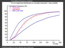
- In hydrology, the log-normal distribution is used to analyze extreme values of such variables as monthly and annual maximum values of daily rainfall and river discharge volumes.[65]
- The image on the right, made with CumFreq, illustrates an example of fitting the log-normal distribution to ranked annually maximum one-day rainfalls showing also the 90% confidence belt based on the binomial distribution.[66]
- The rainfall data are represented by plotting positions as part of a cumulative frequency analysis.
Social sciences and demographics edit
- In economics, there is evidence that the income of 97%–99% of the population is distributed log-normally.[67] (The distribution of higher-income individuals follows a Pareto distribution).[68]
- If an income distribution follows a log-normal distribution with standard deviation , then the Gini coefficient, commonly use to evaluate income inequality, can be computed as where is the error function, since , where is the cumulative distribution function of a standard normal distribution.
- In finance, in particular the Black–Scholes model, changes in the logarithm of exchange rates, price indices, and stock market indices are assumed normal[69] (these variables behave like compound interest, not like simple interest, and so are multiplicative). However, some mathematicians such as Benoit Mandelbrot have argued [70] that log-Lévy distributions, which possesses heavy tails would be a more appropriate model, in particular for the analysis for stock market crashes. Indeed, stock price distributions typically exhibit a fat tail.[71] The fat tailed distribution of changes during stock market crashes invalidate the assumptions of the central limit theorem.
- In scientometrics, the number of citations to journal articles and patents follows a discrete log-normal distribution.[72][73]
- City sizes (population) satisfy Gibrat's Law.[74] The growth process of city sizes is proportionate and invariant with respect to size. From the central limit theorem therefore, the log of city size is normally distributed.
- The number of sexual partners appears to be best described by a log-normal distribution.[75]


Technology edit
- In reliability analysis, the log-normal distribution is often used to model times to repair a maintainable system.[76]
- In wireless communication, "the local-mean power expressed in logarithmic values, such as dB or neper, has a normal (i.e., Gaussian) distribution."[77] Also, the random obstruction of radio signals due to large buildings and hills, called shadowing, is often modeled as a log-normal distribution.
- Particle size distributions produced by comminution with random impacts, such as in ball milling.[78]
- The file size distribution of publicly available audio and video data files (MIME types) follows a log-normal distribution over five orders of magnitude.[79]
- File sizes of 140 million files on personal computers running the Windows OS, collected in 1999.[80][49]
- Sizes of text-based emails (1990s) and multimedia-based emails (2000s).[49]
- In computer networks and Internet traffic analysis, log-normal is shown as a good statistical model to represent the amount of traffic per unit time. This has been shown by applying a robust statistical approach on a large groups of real Internet traces. In this context, the log-normal distribution has shown a good performance in two main use cases: (1) predicting the proportion of time traffic will exceed a given level (for service level agreement or link capacity estimation) i.e. link dimensioning based on bandwidth provisioning and (2) predicting 95th percentile pricing.[81]
- in physical testing when the test produces a time-to-failure of an item under specified conditions, the data is often best analyzed using a lognormal distribution.[82][83]
See also edit
Notes edit
- ^ Norton, Matthew; Khokhlov, Valentyn; Uryasev, Stan (2019). "Calculating CVaR and bPOE for common probability distributions with application to portfolio optimization and density estimation" (PDF). Annals of Operations Research. 299 (1–2). Springer: 1281–1315. arXiv:1811.11301. doi:10.1007/s10479-019-03373-1. S2CID 254231768. Archived (PDF) from the original on 2021-04-18. Retrieved 2023-02-27 – via stonybrook.edu.
- ^ a b c d Weisstein, Eric W. "Log Normal Distribution". mathworld.wolfram.com. Retrieved 2020-09-13.
- ^ a b "1.3.6.6.9. Lognormal Distribution". www.itl.nist.gov. U.S. National Institute of Standards and Technology (NIST). Retrieved 2020-09-13.
- ^ a b c d e Johnson, Norman L.; Kotz, Samuel; Balakrishnan, N. (1994), "14: Lognormal Distributions", Continuous univariate distributions. Vol. 1, Wiley Series in Probability and Mathematical Statistics: Applied Probability and Statistics (2nd ed.), New York: John Wiley & Sons, ISBN 978-0-471-58495-7, MR 1299979
- ^ Park, Sung Y.; Bera, Anil K. (2009). "Maximum entropy autoregressive conditional heteroskedasticity model" (PDF). Journal of Econometrics. 150 (2): 219–230, esp. Table 1, p. 221. CiteSeerX 10.1.1.511.9750. doi:10.1016/j.jeconom.2008.12.014. Archived from the original (PDF) on 2016-03-07. Retrieved 2011-06-02.
- ^ Tarmast, Ghasem (2001). Multivariate Log–Normal Distribution (PDF). ISI Proceedings: 53rd Session. Seoul. Archived (PDF) from the original on 2013-07-19.
- ^ Halliwell, Leigh (2015). The Lognormal Random Multivariate (PDF). Casualty Actuarial Society E-Forum, Spring 2015. Arlington, VA. Archived (PDF) from the original on 2015-09-30.
- ^ Heyde, CC. (2010), "On a Property of the Lognormal Distribution", Journal of the Royal Statistical Society, Series B, vol. 25, no. 2, pp. 392–393, doi:10.1007/978-1-4419-5823-5_6, ISBN 978-1-4419-5822-8
- ^ Billingsley, Patrick (2012). Probability and Measure (Anniversary ed.). Hoboken, N.J.: Wiley. p. 415. ISBN 978-1-118-12237-2. OCLC 780289503.
- ^ a b Holgate, P. (1989). "The lognormal characteristic function, vol. 18, pp. 4539–4548, 1989". Communications in Statistics - Theory and Methods. 18 (12): 4539–4548. doi:10.1080/03610928908830173.
- ^ Barakat, R. (1976). "Sums of independent lognormally distributed random variables". Journal of the Optical Society of America. 66 (3): 211–216. Bibcode:1976JOSA...66..211B. doi:10.1364/JOSA.66.000211.
- ^ Barouch, E.; Kaufman, GM.; Glasser, ML. (1986). "On sums of lognormal random variables" (PDF). Studies in Applied Mathematics. 75 (1): 37–55. doi:10.1002/sapm198675137. hdl:1721.1/48703.
- ^ Leipnik, Roy B. (January 1991). "On Lognormal Random Variables: I – The Characteristic Function" (PDF). Journal of the Australian Mathematical Society, Series B. 32 (3): 327–347. doi:10.1017/S0334270000006901.
- ^ S. Asmussen, J.L. Jensen, L. Rojas-Nandayapa (2016). "On the Laplace transform of the Lognormal distribution", Methodology and Computing in Applied Probability 18 (2), 441-458. Thiele report 6 (13).
- ^ a b c Das, Abhranil (2021). "A method to integrate and classify normal distributions". Journal of Vision. 21 (10): 1. arXiv:2012.14331. doi:10.1167/jov.21.10.1. PMC 8419883. PMID 34468706.
- ^ a b Kirkwood, Thomas BL (Dec 1979). "Geometric means and measures of dispersion". Biometrics. 35 (4): 908–9. JSTOR 2530139.
- ^ Limpert, E; Stahel, W; Abbt, M (2001). "Lognormal distributions across the sciences: keys and clues". BioScience. 51 (5): 341–352. doi:10.1641/0006-3568(2001)051[0341:LNDATS]2.0.CO;2.
- ^ a b Heil P, Friedrich B (2017). "Onset-Duration Matching of Acoustic Stimuli Revisited: Conventional Arithmetic vs. Proposed Geometric Measures of Accuracy and Precision". Frontiers in Psychology. 7: 2013. doi:10.3389/fpsyg.2016.02013. PMC 5216879. PMID 28111557.
- ^ Sawant, S.; Mohan, N. (2011) "FAQ: Issues with Efficacy Analysis of Clinical Trial Data Using SAS" Archived 24 August 2011 at the Wayback Machine, PharmaSUG2011, Paper PO08
- ^ Schiff, MH; et al. (2014). "Head-to-head, randomised, crossover study of oral versus subcutaneous methotrexate in patients with rheumatoid arthritis: drug-exposure limitations of oral methotrexate at doses >=15 mg may be overcome with subcutaneous administration". Ann Rheum Dis. 73 (8): 1–3. doi:10.1136/annrheumdis-2014-205228. PMC 4112421. PMID 24728329.
- ^ Daly, Leslie E.; Bourke, Geoffrey Joseph (2000). Interpretation and Uses of Medical Statistics (5th ed.). Oxford, UK: Wiley-Blackwell. p. 89. doi:10.1002/9780470696750. ISBN 978-0-632-04763-5. PMC 1059583; print edition. Online eBook ISBN 9780470696750
- ^ "ProbOnto". Retrieved 1 July 2017.
- ^ Swat, MJ; Grenon, P; Wimalaratne, S (2016). "ProbOnto: ontology and knowledge base of probability distributions". Bioinformatics. 32 (17): 2719–21. doi:10.1093/bioinformatics/btw170. PMC 5013898. PMID 27153608.
- ^ a b Forbes et al. Probability Distributions (2011), John Wiley & Sons, Inc.
- ^ Lunn, D. (2012). The BUGS book: a practical introduction to Bayesian analysis. Texts in statistical science. CRC Press.
- ^ Limpert, E.; Stahel, W. A.; Abbt, M. (2001). "Log-normal distributions across the sciences: Keys and clues". BioScience. 51 (5): 341–352. doi:10.1641/0006-3568(2001)051[0341:LNDATS]2.0.CO;2.
- ^ Nyberg, J.; et al. (2012). "PopED - An extended, parallelized, population optimal design tool". Comput Methods Programs Biomed. 108 (2): 789–805. doi:10.1016/j.cmpb.2012.05.005. PMID 22640817.
- ^ Retout, S; Duffull, S; Mentré, F (2001). "Development and implementation of the population Fisher information matrix for the evaluation of population pharmacokinetic designs". Comp Meth Pro Biomed. 65 (2): 141–151. doi:10.1016/S0169-2607(00)00117-6. PMID 11275334.
- ^ The PopED Development Team (2016). PopED Manual, Release version 2.13. Technical report, Uppsala University.
- ^ ProbOnto website, URL: http://probonto.org
- ^ Damgaard, Christian; Weiner, Jacob (2000). "Describing inequality in plant size or fecundity". Ecology. 81 (4): 1139–1142. doi:10.1890/0012-9658(2000)081[1139:DIIPSO]2.0.CO;2.
- ^ Rossman, Lewis A (July 1990). "Design stream flows based on harmonic means". Journal of Hydraulic Engineering. 116 (7): 946–950. doi:10.1061/(ASCE)0733-9429(1990)116:7(946).
- ^ Thorin, Olof (1977). "On the infinite divisibility of the lognormal distribution". Scandinavian Actuarial Journal. 1977 (3): 121–148. doi:10.1080/03461238.1977.10405635. ISSN 0346-1238.
- ^ a b Gao, Xin (2009). "Asymptotic Behavior of Tail Density for Sum of Correlated Lognormal Variables". International Journal of Mathematics and Mathematical Sciences. 2009: 1–28. doi:10.1155/2009/630857.
- ^ Asmussen, S.; Rojas-Nandayapa, L. (2008). "Asymptotics of Sums of Lognormal Random Variables with Gaussian Copula" (PDF). Statistics and Probability Letters. 78 (16): 2709–2714. doi:10.1016/j.spl.2008.03.035.
- ^ Marlow, NA. (Nov 1967). "A normal limit theorem for power sums of independent normal random variables". Bell System Technical Journal. 46 (9): 2081–2089. doi:10.1002/j.1538-7305.1967.tb04244.x.
- ^ Botev, Z. I.; L'Ecuyer, P. (2017). "Accurate computation of the right tail of the sum of dependent log-normal variates". 2017 Winter Simulation Conference (WSC), 3rd–6th Dec 2017. Las Vegas, NV, USA: IEEE. pp. 1880–1890. arXiv:1705.03196. doi:10.1109/WSC.2017.8247924. ISBN 978-1-5386-3428-8.
- ^ Asmussen, A.; Goffard, P.-O.; Laub, P. J. (2016). "Orthonormal polynomial expansions and lognormal sum densities". arXiv:1601.01763v1 [math.PR].
- ^ Sangal, B.; Biswas, A. (1970). "The 3-Parameter Lognormal Distribution Applications in Hydrology". Water Resources Research. 6 (2): 505–515. doi:10.1029/WR006i002p00505.
- ^ Johnson, N. L. (1949). "Systems of Frequency Curves Generated by Methods of Translation". Biometrika. 36 (1/2): 149–176. doi:10.2307/2332539. JSTOR 2332539. PMID 18132090.
- ^ Swamee, P. K. (2002). "Near Lognormal Distribution". Journal of Hydrologic Engineering. 7 (6): 441–444. doi:10.1061/(ASCE)1084-0699(2002)7:6(441).
- ^ a b Wu, Ziniu; Li, Juan; Bai, Chenyuan (2017). "Scaling Relations of Lognormal Type Growth Process with an Extremal Principle of Entropy". Entropy. 19 (56): 1–14. Bibcode:2017Entrp..19...56W. doi:10.3390/e19020056.
- ^ Wu, Zi-Niu (2003). "Prediction of the size distribution of secondary ejected droplets by crown splashing of droplets impinging on a solid wall". Probabilistic Engineering Mechanics. 18 (3): 241–249. doi:10.1016/S0266-8920(03)00028-6.
- ^ Wang, WenBin; Wu, ZiNiu; Wang, ChunFeng; Hu, RuiFeng (2013). "Modelling the spreading rate of controlled communicable epidemics through an entropy-based thermodynamic model". Science China Physics, Mechanics and Astronomy. 56 (11): 2143–2150. arXiv:1304.5603. Bibcode:2013SCPMA..56.2143W. doi:10.1007/s11433-013-5321-0. ISSN 1674-7348. PMC 7111546. PMID 32288765.
- ^ Bloetscher, Frederick (2019). "Using predictive Bayesian Monte Carlo- Markov Chain methods to provide a probabilistic solution for the Drake equation". Acta Astronautica. 155: 118–130. Bibcode:2019AcAau.155..118B. doi:10.1016/j.actaastro.2018.11.033. S2CID 117598888.
- ^ Sutton, John (Mar 1997). "Gibrat's Legacy". Journal of Economic Literature. 32 (1): 40–59. JSTOR 2729692.
- ^ a b c Limpert, Eckhard; Stahel, Werner A.; Abbt, Markus (2001). "Log-normal Distributions across the Sciences: Keys and Clues". BioScience. 51 (5): 341. doi:10.1641/0006-3568(2001)051[0341:LNDATS]2.0.CO;2. ISSN 0006-3568.
- ^ a b Buzsáki, György; Mizuseki, Kenji (2017-01-06). "The log-dynamic brain: how skewed distributions affect network operations". Nature Reviews. Neuroscience. 15 (4): 264–278. doi:10.1038/nrn3687. ISSN 1471-003X. PMC 4051294. PMID 24569488.
- ^ a b c Pawel, Sobkowicz; et al. (2013). "Lognormal distributions of user post lengths in Internet discussions - a consequence of the Weber-Fechner law?". EPJ Data Science.
- ^ Yin, Peifeng; Luo, Ping; Lee, Wang-Chien; Wang, Min (2013). Silence is also evidence: interpreting dwell time for recommendation from psychological perspective. ACM International Conference on KDD.
- ^ "What is the average length of a game of chess?". chess.stackexchange.com. Retrieved 14 April 2018.
- ^ Huxley, Julian S. (1932). Problems of relative growth. London. ISBN 978-0-486-61114-3. OCLC 476909537.
- ^ Sartwell, Philip E. "The distribution of incubation periods of infectious disease." American journal of hygiene 51 (1950): 310-318.
- ^ S. K. Chan, Jennifer; Yu, Philip L. H. (2006). "Modelling SARS data using threshold geometric process". Statistics in Medicine. 25 (11): 1826–1839. doi:10.1002/sim.2376. PMID 16345017. S2CID 46599163.
- ^ Ono, Yukiteru; Asai, Kiyoshi; Hamada, Michiaki (2013-01-01). "PBSIM: PacBio reads simulator—toward accurate genome assembly". Bioinformatics. 29 (1): 119–121. doi:10.1093/bioinformatics/bts649. ISSN 1367-4803. PMID 23129296.
- ^ Makuch, Robert W.; D.H. Freeman; M.F. Johnson (1979). "Justification for the lognormal distribution as a model for blood pressure". Journal of Chronic Diseases. 32 (3): 245–250. doi:10.1016/0021-9681(79)90070-5. PMID 429469.
- ^ Lacey, L. F.; Keene, O. N.; Pritchard, J. F.; Bye, A. (1997-01-01). "Common noncompartmental pharmacokinetic variables: are they normally or log-normally distributed?". Journal of Biopharmaceutical Statistics. 7 (1): 171–178. doi:10.1080/10543409708835177. ISSN 1054-3406. PMID 9056596.
- ^ Scheler, Gabriele; Schumann, Johann (2006-10-08). Diversity and stability in neuronal output rates. 36th Society for Neuroscience Meeting, Atlanta.
- ^ Mizuseki, Kenji; Buzsáki, György (2013-09-12). "Preconfigured, skewed distribution of firing rates in the hippocampus and entorhinal cortex". Cell Reports. 4 (5): 1010–1021. doi:10.1016/j.celrep.2013.07.039. ISSN 2211-1247. PMC 3804159. PMID 23994479.
- ^ Wohrer, Adrien; Humphries, Mark D.; Machens, Christian K. (2013-04-01). "Population-wide distributions of neural activity during perceptual decision-making". Progress in Neurobiology. 103: 156–193. doi:10.1016/j.pneurobio.2012.09.004. ISSN 1873-5118. PMC 5985929. PMID 23123501.
- ^ Scheler, Gabriele (2017-07-28). "Logarithmic distributions prove that intrinsic learning is Hebbian". F1000Research. 6: 1222. doi:10.12688/f1000research.12130.2. PMC 5639933. PMID 29071065.
- ^ Morales-Gregorio, Aitor; van Meegen, Alexander; van Albada, Sacha (2023). "Ubiquitous lognormal distribution of neuron densities in mammalian cerebral cortex". Cerebral Cortex. 33 (16): 9439–9449. doi:10.1093/cercor/bhad160. PMC 10438924. PMID 37409647.
- ^ Polizzi, Stefano; Laperrousaz, Bastien; Perez-Reche, Francisco J; Nicolini, Franck E; Satta, Véronique Maguer; Arneodo, Alain; Argoul, Françoise (2018-05-29). "A minimal rupture cascade model for living cell plasticity". New Journal of Physics. 20 (5): 053057. doi:10.1088/1367-2630/aac3c7. hdl:2164/10561. ISSN 1367-2630.
- ^ Ahrens, L. H. (1954-02-01). "The lognormal distribution of the elements (A fundamental law of geochemistry and its subsidiary)". Geochimica et Cosmochimica Acta. 5 (2): 49–73. Bibcode:1954GeCoA...5...49A. doi:10.1016/0016-7037(54)90040-X. ISSN 0016-7037.
- ^ Oosterbaan, R.J. (1994). "6: Frequency and Regression Analysis" (PDF). In Ritzema, H.P. (ed.). Drainage Principles and Applications, Publication 16. Wageningen, The Netherlands: International Institute for Land Reclamation and Improvement (ILRI). pp. 175–224. ISBN 978-90-70754-33-4.
- ^ CumFreq, free software for distribution fitting
- ^ Clementi, Fabio; Gallegati, Mauro (2005) "Pareto's law of income distribution: Evidence for Germany, the United Kingdom, and the United States", EconWPA
- ^ Wataru, Souma (2002-02-22). "Physics of Personal Income". In Takayasu, Hideki (ed.). Empirical Science of Financial Fluctuations: The Advent of Econophysics. Springer. arXiv:cond-mat/0202388. doi:10.1007/978-4-431-66993-7.
- ^ Black, F.; Scholes, M. (1973). "The Pricing of Options and Corporate Liabilities". Journal of Political Economy. 81 (3): 637. doi:10.1086/260062. S2CID 154552078.
- ^ Mandelbrot, Benoit (2004). The (mis-)Behaviour of Markets. Basic Books. ISBN 9780465043552.
- ^ Bunchen, P., Advanced Option Pricing, University of Sydney coursebook, 2007
- ^ Thelwall, Mike; Wilson, Paul (2014). "Regression for citation data: An evaluation of different methods". Journal of Informetrics. 8 (4): 963–971. arXiv:1510.08877. doi:10.1016/j.joi.2014.09.011. S2CID 8338485.
- ^ Sheridan, Paul; Onodera, Taku (2020). "A Preferential Attachment Paradox: How Preferential Attachment Combines with Growth to Produce Networks with Log-normal In-degree Distributions". Scientific Reports. 8 (1): 2811. arXiv:1703.06645. doi:10.1038/s41598-018-21133-2. PMC 5809396. PMID 29434232.
- ^ Eeckhout, Jan (2004). "Gibrat's Law for (All) Cities". American Economic Review. 94 (5): 1429–1451. doi:10.1257/0002828043052303. JSTOR 3592829 – via JSTOR.
- ^ Kault, David (1996). "The Shape of the Distribution of the Number of Sexual Partners". Statistics in Medicine. 15 (2): 221–230. doi:10.1002/(SICI)1097-0258(19960130)15:2<221::AID-SIM148>3.0.CO;2-Q. PMID 8614756.
- ^ O'Connor, Patrick; Kleyner, Andre (2011). Practical Reliability Engineering. John Wiley & Sons. p. 35. ISBN 978-0-470-97982-2.
- ^ "Shadowing". www.WirelessCommunication.NL. Archived from the original on January 13, 2012.
- ^ Dexter, A. R.; Tanner, D. W. (July 1972). "Packing Densities of Mixtures of Spheres with Log-normal Size Distributions". Nature Physical Science. 238 (80): 31–32. Bibcode:1972NPhS..238...31D. doi:10.1038/physci238031a0. ISSN 2058-1106.
- ^ Gros, C; Kaczor, G.; Markovic, D (2012). "Neuropsychological constraints to human data production on a global scale". The European Physical Journal B. 85 (28): 28. arXiv:1111.6849. Bibcode:2012EPJB...85...28G. doi:10.1140/epjb/e2011-20581-3. S2CID 17404692.
- ^ Douceur, John R.; Bolosky, William J. (1999-05-01). "A large-scale study of file-system contents". ACM SIGMETRICS Performance Evaluation Review. 27 (1): 59–70. doi:10.1145/301464.301480. ISSN 0163-5999.
- ^ Alamsar, Mohammed; Parisis, George; Clegg, Richard; Zakhleniuk, Nickolay (2019). "On the Distribution of Traffic Volumes in the Internet and its Implications". arXiv:1902.03853 [cs.NI].
- ^ ASTM D3654, Standard Test Method for Shear Adhesion on Pressure-Sensitive Tapesw
- ^ ASTM D4577, Standard Test Method for Compression Resistance of a container Under Constant Load>\
Further reading edit
- Crow, Edwin L.; Shimizu, Kunio, eds. (1988), Lognormal Distributions, Theory and Applications, Statistics: Textbooks and Monographs, vol. 88, New York: Marcel Dekker, Inc., pp. xvi+387, ISBN 978-0-8247-7803-3, MR 0939191, Zbl 0644.62014
- Aitchison, J. and Brown, J.A.C. (1957) The Lognormal Distribution, Cambridge University Press.
- Limpert, E; Stahel, W; Abbt, M (2001). "Lognormal distributions across the sciences: keys and clues". BioScience. 51 (5): 341–352. doi:10.1641/0006-3568(2001)051[0341:LNDATS]2.0.CO;2.
- Holgate, P. (1989). "The lognormal characteristic function". Communications in Statistics - Theory and Methods. 18 (12): 4539–4548. doi:10.1080/03610928908830173.
- Brooks, Robert; Corson, Jon; Donal, Wales (1994). "The Pricing of Index Options When the Underlying Assets All Follow a Lognormal Diffusion". Advances in Futures and Options Research. 7. SSRN 5735.
External links edit
- The normal distribution is the log-normal distribution