


Summary
In probability theory and statistics, the logistic distribution is a continuous probability distribution. Its cumulative distribution function is the logistic function, which appears in logistic regression and feedforward neural networks. It resembles the normal distribution in shape but has heavier tails (higher kurtosis). The logistic distribution is a special case of the Tukey lambda distribution.
|
Probability density function 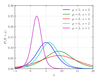 | |||
|
Cumulative distribution function 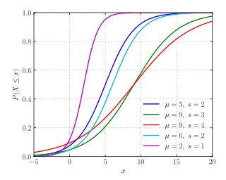 | |||
| Parameters |
location (real) scale (real) | ||
|---|---|---|---|
| Support | |||
| CDF | |||
| Quantile | |||
| Mean | |||
| Median | |||
| Mode | |||
| Variance | |||
| Skewness | |||
| Excess kurtosis | |||
| Entropy | |||
| MGF |
for and is the Beta function | ||
| CF | |||
| Expected shortfall |
where is the binary entropy function[1] | ||


Specification edit
Probability density function edit
When the location parameter μ is 0 and the scale parameter s is 1, then the probability density function of the logistic distribution is given by
![{\displaystyle {\begin{aligned}f(x;0,1)&={\frac {e^{-x}}{(1+e^{-x})^{2}}}\\[4pt]&={\frac {1}{(e^{x/2}+e^{-x/2})^{2}}}\\[5pt]&={\frac {1}{4}}\operatorname {sech} ^{2}\left({\frac {x}{2}}\right).\end{aligned}}}](https://wikimedia.org/api/rest_v1/media/math/render/svg/754aa5c354f6af79cac3f2942b7d423cb0545ca0)
Thus in general the density is:
![{\displaystyle {\begin{aligned}f(x;\mu ,s)&={\frac {e^{-(x-\mu )/s}}{s\left(1+e^{-(x-\mu )/s}\right)^{2}}}\\[4pt]&={\frac {1}{s\left(e^{(x-\mu )/(2s)}+e^{-(x-\mu )/(2s)}\right)^{2}}}\\[4pt]&={\frac {1}{4s}}\operatorname {sech} ^{2}\left({\frac {x-\mu }{2s}}\right).\end{aligned}}}](https://wikimedia.org/api/rest_v1/media/math/render/svg/bb846bd4f193547bf2fefaa813702f0b19d19ce0)
Because this function can be expressed in terms of the square of the hyperbolic secant function "sech", it is sometimes referred to as the sech-square(d) distribution.[2] (See also: hyperbolic secant distribution).
Cumulative distribution function edit
The logistic distribution receives its name from its cumulative distribution function, which is an instance of the family of logistic functions. The cumulative distribution function of the logistic distribution is also a scaled version of the hyperbolic tangent.

In this equation μ is the mean, and s is a scale parameter proportional to the standard deviation.
Quantile function edit
The inverse cumulative distribution function (quantile function) of the logistic distribution is a generalization of the logit function. Its derivative is called the quantile density function. They are defined as follows:


Alternative parameterization edit
An alternative parameterization of the logistic distribution can be derived by expressing the scale parameter, , in terms of the standard deviation, , using the substitution , where . The alternative forms of the above functions are reasonably straightforward.


Applications edit
The logistic distribution—and the S-shaped pattern of its cumulative distribution function (the logistic function) and quantile function (the logit function)—have been extensively used in many different areas.
Logistic regression edit
One of the most common applications is in logistic regression, which is used for modeling categorical dependent variables (e.g., yes-no choices or a choice of 3 or 4 possibilities), much as standard linear regression is used for modeling continuous variables (e.g., income or population). Specifically, logistic regression models can be phrased as latent variable models with error variables following a logistic distribution. This phrasing is common in the theory of discrete choice models, where the logistic distribution plays the same role in logistic regression as the normal distribution does in probit regression. Indeed, the logistic and normal distributions have a quite similar shape. However, the logistic distribution has heavier tails, which often increases the robustness of analyses based on it compared with using the normal distribution.
Physics edit
The PDF of this distribution has the same functional form as the derivative of the Fermi function. In the theory of electron properties in semiconductors and metals, this derivative sets the relative weight of the various electron energies in their contributions to electron transport. Those energy levels whose energies are closest to the distribution's "mean" (Fermi level) dominate processes such as electronic conduction, with some smearing induced by temperature.[3]: 34 Note however that the pertinent probability distribution in Fermi–Dirac statistics is actually a simple Bernoulli distribution, with the probability factor given by the Fermi function.
The logistic distribution arises as limit distribution of a finite-velocity damped random motion described by a telegraph process in which the random times between consecutive velocity changes have independent exponential distributions with linearly increasing parameters.[4]
Hydrology edit

In hydrology the distribution of long duration river discharge and rainfall (e.g., monthly and yearly totals, consisting of the sum of 30 respectively 360 daily values) is often thought to be almost normal according to the central limit theorem.[5] The normal distribution, however, needs a numeric approximation. As the logistic distribution, which can be solved analytically, is similar to the normal distribution, it can be used instead. The blue picture illustrates an example of fitting the logistic distribution to ranked October rainfalls—that are almost normally distributed—and it shows the 90% confidence belt based on the binomial distribution. The rainfall data are represented by plotting positions as part of the cumulative frequency analysis.
Chess ratings edit
The United States Chess Federation and FIDE have switched its formula for calculating chess ratings from the normal distribution to the logistic distribution; see the article on Elo rating system (itself based on the normal distribution).
Related distributions edit
- Logistic distribution mimics the sech distribution.
- If then .
- If U(0, 1) then .
- If and independently then .
- If and then (The sum is not a logistic distribution). Note that .
- If X ~ Logistic(μ, s) then exp(X) ~ LogLogistic , and exp(X) + γ ~ shifted log-logistic .
- If X ~ Exponential(1) then


- If X, Y ~ Exponential(1) then

- The metalog distribution is generalization of the logistic distribution, in which power series expansions in terms of are substituted for logistic parameters and . The resulting metalog quantile function is highly shape flexible, has a simple closed form, and can be fit to data with linear least squares.

Derivations edit
Higher-order moments edit
The nth-order central moment can be expressed in terms of the quantile function:
![{\displaystyle {\begin{aligned}\operatorname {E} [(X-\mu )^{n}]&=\int _{-\infty }^{\infty }(x-\mu )^{n}\,dF(x)\\&=\int _{0}^{1}{\big (}Q(p)-\mu {\big )}^{n}\,dp=s^{n}\int _{0}^{1}\left[\ln \!\left({\frac {p}{1-p}}\right)\right]^{n}\,dp.\end{aligned}}}](https://wikimedia.org/api/rest_v1/media/math/render/svg/13fbb4b93932c1c8b46305452c4285326774aeec)
This integral is well-known[6] and can be expressed in terms of Bernoulli numbers:
![{\displaystyle \operatorname {E} [(X-\mu )^{n}]=s^{n}\pi ^{n}(2^{n}-2)\cdot |B_{n}|.}](https://wikimedia.org/api/rest_v1/media/math/render/svg/36c3b6137df258b36cca0d6122cf65db40447a51)
See also edit
Notes edit
- ^ Norton, Matthew; Khokhlov, Valentyn; Uryasev, Stan (2019). "Calculating CVaR and bPOE for common probability distributions with application to portfolio optimization and density estimation" (PDF). Annals of Operations Research. 299 (1–2). Springer: 1281–1315. doi:10.1007/s10479-019-03373-1. Retrieved 2023-02-27.
- ^ Johnson, Kotz & Balakrishnan (1995, p.116).
- ^ Davies, John H. (1998). The Physics of Low-dimensional Semiconductors: An Introduction. Cambridge University Press. ISBN 9780521484916.
- ^ A. Di Crescenzo, B. Martinucci (2010) "A damped telegraph random process with logistic stationary distribution", J. Appl. Prob., vol. 47, pp. 84–96.
- ^ Ritzema, H.P., ed. (1994). Frequency and Regression Analysis. Chapter 6 in: Drainage Principles and Applications, Publication 16, International Institute for Land Reclamation and Improvement (ILRI), Wageningen, The Netherlands. pp. 175–224. ISBN 90-70754-33-9.
- ^ OEIS: A001896
References edit
- John S. deCani & Robert A. Stine (1986). "A note on deriving the information matrix for a logistic distribution". The American Statistician. 40. American Statistical Association: 220–222. doi:10.2307/2684541.
- N., Balakrishnan (1992). Handbook of the Logistic Distribution. Marcel Dekker, New York. ISBN 0-8247-8587-8.
- Johnson, N. L.; Kotz, S.; N., Balakrishnan (1995). Continuous Univariate Distributions. Vol. 2 (2nd ed.). ISBN 0-471-58494-0.
- Modis, Theodore (1992) Predictions: Society's Telltale Signature Reveals the Past and Forecasts the Future, Simon & Schuster, New York. ISBN 0-671-75917-5