In the moment distribution method, every joint of the structure to be analysed is fixed so as to develop the fixed-end moments. Then each fixed joint is sequentially released and the fixed-end moments (which by the time of release are not in equilibrium) are distributed to adjacent members until equilibrium is achieved. The moment distribution method in mathematical terms can be demonstrated as the process of solving a set of simultaneous equations by means of iteration.

The moment distribution method falls into the category of displacement method of structural analysis.

In order to apply the moment distribution method to analyse a structure, the following things must be considered.

Fixed end moments edit

Fixed end moments are the moments produced at member ends by external loads.

Bending stiffness edit

The bending stiffness (EI/L) of a member is represented as the flexural rigidity of the member (product of the modulus of elasticity (E) and the second moment of area (I)) divided by the length (L) of the member. What is needed in the moment distribution method is not the specific values but the ratios of bending stiffnesses between all members.

Distribution factors edit

When a joint is being released and begins to rotate under the unbalanced moment, resisting forces develop at each member framed together at the joint. Although the total resistance is equal to the unbalanced moment, the magnitudes of resisting forces developed at each member differ by the members' bending stiffness. Distribution factors can be defined as the proportions of the unbalanced moments carried by each of the members. In mathematical terms, the distribution factor of member ${\displaystyle k}$  framed at joint ${\displaystyle j}$  is given as:

${\displaystyle D_{jk}={\frac {\frac {E_{k}I_{k}}{L_{k}}}{\sum _{i=1}^{i=n}{\frac {E_{i}I_{i}}{L_{i}}}}}}$ 

where n is the number of members framed at the joint.

Carryover factors edit

When a joint is released, balancing moment occurs to counterbalance the unbalanced moment. The balancing moment is initially the same as the fixed-end moment. This balancing moment is then carried over to the member's other end. The ratio of the carried-over moment at the other end to the fixed-end moment of the initial end is the carryover factor.

Determination of carryover factors edit

Let one end (end A) of a fixed beam be released and applied a moment ${\displaystyle M_{A}}$  while the other end (end B) remains fixed. This will cause end A to rotate through an angle ${\displaystyle \theta _{A}}$ . Once the magnitude of ${\displaystyle M_{B}}$  developed at end B is found, the carryover factor of this member is given as the ratio of ${\displaystyle M_{B}}$  over ${\displaystyle M_{A}}$ :

${\displaystyle C_{AB}={\frac {M_{B}}{M_{A}}}}$ 

In case of a beam of length L with constant cross-section whose flexural rigidity is ${\displaystyle EI}$ ,

${\displaystyle M_{A}=4{\frac {EI}{L}}\theta _{A}+2{\frac {EI}{L}}\theta _{B}=4{\frac {EI}{L}}\theta _{A}}$ 

${\displaystyle M_{B}=2{\frac {EI}{L}}\theta _{A}+4{\frac {EI}{L}}\theta _{B}=2{\frac {EI}{L}}\theta _{A}}$ 

therefore the carryover factor

${\displaystyle C_{AB}={\frac {M_{B}}{M_{A}}}={\frac {1}{2}}}$ 

Sign convention edit

Once a sign convention has been chosen, it has to be maintained for the whole structure. The traditional engineer's sign convention is not used in the calculations of the moment distribution method although the results can be expressed in the conventional way. In the BMD case, the left side moment is clockwise direction and other is anticlockwise direction so the bending is positive and is called sagging.

Framed structure edit

Framed structure with or without sidesway can be analysed using the moment distribution method.

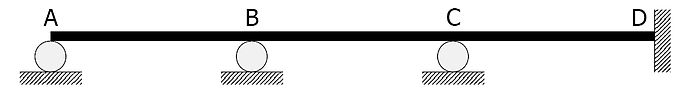
The statically indeterminate beam shown in the figure is to be analysed.

The beam is considered to be three separate members, AB, BC, and CD, connected by fixed end (moment resisting) joints at B and C.

• Members AB, BC, CD have the same span ${\displaystyle L=10\ m}$ .
• Flexural rigidities are EI, 2EI, EI respectively.
• Concentrated load of magnitude ${\displaystyle P=10\ kN}$  acts at a distance ${\displaystyle a=3\ m}$  from the support A.
• Uniform load of intensity ${\displaystyle q=1\ kN/m}$  acts on BC.
• Member CD is loaded at its midspan with a concentrated load of magnitude ${\displaystyle P=10\ kN}$ .

In the following calculations, clockwise moments are positive.

Fixed end moments edit

${\displaystyle M_{AB}^{f}=-{\frac {Pb^{2}a}{L^{2}}}=-{\frac {10\times 7^{2}\times 3}{10^{2}}}=-14.700\ kN\cdot m}$ 

${\displaystyle M_{BA}^{f}={\frac {Pa^{2}b}{L^{2}}}={\frac {10\times 3^{2}\times 7}{10^{2}}}=+6.300\ kN\cdot m}$ 

${\displaystyle M_{BC}^{f}=-{\frac {qL^{2}}{12}}=-{\frac {1\times 10^{2}}{12}}=-8.333\ kN\cdot m}$ 

${\displaystyle M_{CB}^{f}={\frac {qL^{2}}{12}}={\frac {1\times 10^{2}}{12}}=+8.333\ kN\cdot m}$ 

${\displaystyle M_{CD}^{f}=-{\frac {PL}{8}}=-{\frac {10\times 10}{8}}=-12.500\ kN\cdot m}$ 

${\displaystyle M_{DC}^{f}={\frac {PL}{8}}={\frac {10\times 10}{8}}=+12.500\ kN\cdot m}$ 

Bending stiffness and distribution factors edit

The bending stiffness of members AB, BC and CD are ${\displaystyle {\frac {3EI}{L}}}$ , ${\displaystyle {\frac {4\times 2EI}{L}}}$  and ${\displaystyle {\frac {4EI}{L}}}$ , respectively ^{[disputed – discuss]}. Therefore, expressing the results in repeating decimal notation:

${\displaystyle D_{BA}={\frac {\frac {3EI}{L}}{{\frac {3EI}{L}}+{\frac {4\times 2EI}{L}}}}={\frac {\frac {3}{10}}{{\frac {3}{10}}+{\frac {8}{10}}}}={\frac {3}{11}}=0.(27)}$ 

${\displaystyle D_{BC}={\frac {\frac {4\times 2EI}{L}}{{\frac {3EI}{L}}+{\frac {4\times 2EI}{L}}}}={\frac {\frac {8}{10}}{{\frac {3}{10}}+{\frac {8}{10}}}}={\frac {8}{11}}=0.(72)}$ 

${\displaystyle D_{CB}={\frac {\frac {4\times 2EI}{L}}{{\frac {4\times 2EI}{L}}+{\frac {4EI}{L}}}}={\frac {\frac {8}{10}}{{\frac {8}{10}}+{\frac {4}{10}}}}={\frac {8}{12}}=0.(66)}$ 

${\displaystyle D_{CD}={\frac {\frac {4EI}{L}}{{\frac {4\times 2EI}{L}}+{\frac {4EI}{L}}}}={\frac {\frac {4}{10}}{{\frac {8}{10}}+{\frac {4}{10}}}}={\frac {4}{12}}=0.(33)}$ 

The distribution factors of joints A and D are ${\displaystyle D_{AB}=1}$  and ${\displaystyle D_{DC}=0}$ .

Carryover factors edit

The carryover factors are ${\displaystyle {\frac {1}{2}}}$ , except for the carryover factor from D (fixed support) to C which is zero.

Moment distribution edit

Numbers in grey are balanced moments; arrows ( → / ← ) represent the carry-over of moment from one end to the other end of a member.* Step 1: As joint A is released, balancing moment of magnitude equal to the fixed end moment ${\displaystyle M_{AB}^{f}=14.700\mathrm {\,kN\,m} }$  develops and is carried-over from joint A to joint B.* Step 2: The unbalanced moment at joint B now is the summation of the fixed end moments ${\displaystyle M_{BA}^{f}}$ , ${\displaystyle M_{BC}^{f}}$  and the carry-over moment from joint A. This unbalanced moment is distributed to members BA and BC in accordance with the distribution factors ${\displaystyle D_{BA}=0.2727}$  and ${\displaystyle D_{BC}=0.7273}$ . Step 2 ends with carry-over of balanced moment ${\displaystyle M_{BC}=3.867\mathrm {\,kN\,m} }$  to joint C. Joint A is a roller support which has no rotational restraint, so moment carryover from joint B to joint A is zero.* Step 3: The unbalanced moment at joint C now is the summation of the fixed end moments ${\displaystyle M_{CB}^{f}}$ , ${\displaystyle M_{CD}^{f}}$  and the carryover moment from joint B. As in the previous step, this unbalanced moment is distributed to each member and then carried over to joint D and back to joint B. Joint D is a fixed support and carried-over moments to this joint will not be distributed nor be carried over to joint C.* Step 4: Joint B still has balanced moment which was carried over from joint C in step 3. Joint B is released once again to induce moment distribution and to achieve equilibrium.* Steps 5 - 10: Joints are released and fixed again until every joint has unbalanced moments of size zero or neglectably small in required precision. Arithmetically summing all moments in each respective columns gives the final moment values.

Result edit

• Moments at joints determined by the moment distribution method

${\displaystyle M_{A}=0\ kN\cdot m}$ 

${\displaystyle M_{B}=-11.569\ kN\cdot m}$ 

${\displaystyle M_{C}=-10.186\ kN\cdot m}$ 

${\displaystyle M_{D}=-13.657\ kN\cdot m}$ 

The conventional engineer's sign convention is used here, i.e. positive moments cause elongation at the bottom part of a beam member.

For comparison purposes, the following are the results generated using a matrix method. Note that in the analysis above, the iterative process was carried to >0.01 precision. The fact that the matrix analysis results and the moment distribution analysis results match to 0.001 precision is mere coincidence.

• Moments at joints determined by the matrix method

${\displaystyle M_{A}=0\ kN\cdot m}$ 

${\displaystyle M_{B}=-11.569\ kN\cdot m}$ 

${\displaystyle M_{C}=-10.186\ kN\cdot m}$ 

${\displaystyle M_{D}=-13.657\ kN\cdot m}$ 

Note that the moment distribution method only determines the moments at the joints. Developing complete bending moment diagrams require additional calculations using the determined joint moments and internal section equilibrium.

Result via displacements method edit

As the Hardy Cross method provides only approximate results, with a margin of error inversely proportionate to the number of iterations, it is important^{[citation needed]} to have an idea of how accurate this method might be. With this in mind, here is the result obtained by using an exact method: the displacement method

For this, the displacements method equation assumes the following form:

${\displaystyle \left[K\right]\left\{d\right\}=\left\{-f\right\}}$ 

For the structure described in this example, the stiffness matrix is as follows:

${\displaystyle \left[K\right]={\begin{bmatrix}3{\frac {EI}{L}}+4{\frac {2EI}{L}}&2{\frac {2EI}{L}}\\2{\frac {2EI}{L}}&4{\frac {2EI}{L}}+4{\frac {EI}{L}}\end{bmatrix}}}$ 

The equivalent nodal force vector:

${\displaystyle \left\{f\right\}^{T}=\left\{-P{\frac {ab(L+a)}{2L^{2}}}+q{\frac {L^{2}}{12}},-q{\frac {L^{2}}{12}}+P{\frac {L}{8}}\right\}}$ 

Replacing the values presented above in the equation and solving it for ${\displaystyle \left\{d\right\}}$  leads to the following result:

${\displaystyle \left\{d\right\}^{T}=\left\{6.9368;-5.7845\right\}}$ 

Hence, the moments evaluated in node B are as follows:

${\displaystyle M_{BA}=3{\frac {EI}{L}}d_{1}-P{\frac {ab(L+a)}{2L^{2}}}=-11.569}$ 

${\displaystyle M_{BC}=-4{\frac {2EI}{L}}d_{1}-2{\frac {2EI}{L}}d_{2}-q{\frac {L^{2}}{12}}=-11.569}$ 

The moments evaluated in node C are as follows:

${\displaystyle M_{CB}=2{\frac {2EI}{L}}d_{1}+4{\frac {2EI}{L}}d_{2}-q{\frac {L^{2}}{12}}=-10.186}$ 

${\displaystyle M_{CD}=-4{\frac {EI}{L}}d_{2}-P{\frac {L}{8}}=-10.186}$ 

• Finite element method
• Slope deflection method

• Błaszkowiak, Stanisław; Zbigniew Kączkowski (1966). Iterative Methods in Structural Analysis. Pergamon Press, Państwowe Wydawnictwo Naukowe.
• Norris, Charles Head; John Benson Wilbur; Senol Utku (1976). Elementary Structural Analysis (3rd ed.). McGraw-Hill. pp. 327–345. ISBN 0-07-047256-4.
• McCormac, Jack C.; Nelson, James K. Jr. (1997). Structural Analysis: A Classical and Matrix Approach (2nd ed.). Addison-Wesley. pp. 488–538. ISBN 0-673-99753-7.
• Yang, Chang-hyeon (2001-01-10). Structural Analysis (in Korean) (4th ed.). Seoul: Cheong Moon Gak Publishers. pp. 391–422. ISBN 89-7088-709-1. Archived from the original on 2007-10-08. Retrieved 2007-08-31.
• Volokh, K.Y. (2002). "On foundations of the Hardy Cross method". International Journal of Solids and Structures. 39 (16). International Journal of Solids and Structures, volume 39, issue 16, August 2002, Pages 4197-4200: 4197–4200. doi:10.1016/S0020-7683(02)00345-1.