


Summary
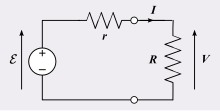
Ohm's law states that the electric current through a conductor between two points is directly proportional to the voltage across the two points. Introducing the constant of proportionality, the resistance,[1] one arrives at the three mathematical equations used to describe this relationship:[2]


where I is the current through the conductor, V is the voltage measured across the conductor and R is the resistance of the conductor. More specifically, Ohm's law states that the R in this relation is constant, independent of the current.[3] If the resistance is not constant, the previous equation cannot be called Ohm's law, but it can still be used as a definition of static/DC resistance.[4] Ohm's law is an empirical relation which accurately describes the conductivity of the vast majority of electrically conductive materials over many orders of magnitude of current. However some materials do not obey Ohm's law; these are called non-ohmic.
The law was named after the German physicist Georg Ohm, who, in a treatise published in 1827, described measurements of applied voltage and current through simple electrical circuits containing various lengths of wire. Ohm explained his experimental results by a slightly more complex equation than the modern form above (see § History below).
In physics, the term Ohm's law is also used to refer to various generalizations of the law; for example the vector form of the law used in electromagnetics and material science:

where J is the current density at a given location in a resistive material, E is the electric field at that location, and σ (sigma) is a material-dependent parameter called the conductivity. This reformulation of Ohm's law is due to Gustav Kirchhoff.[5]
History edit
In January 1781, before Georg Ohm's work, Henry Cavendish experimented with Leyden jars and glass tubes of varying diameter and length filled with salt solution. He measured the current by noting how strong a shock he felt as he completed the circuit with his body. Cavendish wrote that the "velocity" (current) varied directly as the "degree of electrification" (voltage). He did not communicate his results to other scientists at the time,[6] and his results were unknown until James Clerk Maxwell published them in 1879.[7]
Francis Ronalds delineated "intensity" (voltage) and "quantity" (current) for the dry pile—a high voltage source—in 1814 using a gold-leaf electrometer. He found for a dry pile that the relationship between the two parameters was not proportional under certain meteorological conditions.[8][9]
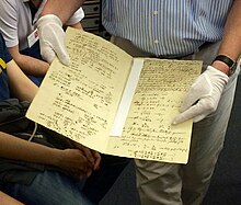
Ohm did his work on resistance in the years 1825 and 1826, and published his results in 1827 as the book Die galvanische Kette, mathematisch bearbeitet ("The galvanic circuit investigated mathematically").[10] He drew considerable inspiration from Joseph Fourier's work on heat conduction in the theoretical explanation of his work. For experiments, he initially used voltaic piles, but later used a thermocouple as this provided a more stable voltage source in terms of internal resistance and constant voltage. He used a galvanometer to measure current, and knew that the voltage between the thermocouple terminals was proportional to the junction temperature. He then added test wires of varying length, diameter, and material to complete the circuit. He found that his data could be modeled through the equation

In modern notation we would write,


Ohm's law was probably the most important of the early quantitative descriptions of the physics of electricity. We consider it almost obvious today. When Ohm first published his work, this was not the case; critics reacted to his treatment of the subject with hostility. They called his work a "web of naked fancies"[11] and the Minister of Education proclaimed that "a professor who preached such heresies was unworthy to teach science."[12] The prevailing scientific philosophy in Germany at the time asserted that experiments need not be performed to develop an understanding of nature because nature is so well ordered, and that scientific truths may be deduced through reasoning alone.[13] Also, Ohm's brother Martin, a mathematician, was battling the German educational system. These factors hindered the acceptance of Ohm's work, and his work did not become widely accepted until the 1840s. However, Ohm received recognition for his contributions to science well before he died.
In the 1850s, Ohm's law was widely known and considered proved. Alternatives such as "Barlow's law", were discredited, in terms of real applications to telegraph system design, as discussed by Samuel F. B. Morse in 1855.[14]
The electron was discovered in 1897 by J. J. Thomson, and it was quickly realized that it was the particle (charge carrier) that carried electric currents in electric circuits. In 1900, the first (classical) model of electrical conduction, the Drude model, was proposed by Paul Drude, which finally gave a scientific explanation for Ohm's law. In this model, a solid conductor consists of a stationary lattice of atoms (ions), with conduction electrons moving randomly in it. A voltage across a conductor causes an electric field, which accelerates the electrons in the direction of the electric field, causing a drift of electrons which is the electric current. However the electrons collide with atoms which causes them to scatter and randomizes their motion, thus converting kinetic energy to heat (thermal energy). Using statistical distributions, it can be shown that the average drift velocity of the electrons, and thus the current, is proportional to the electric field, and thus the voltage, over a wide range of voltages.
The development of quantum mechanics in the 1920s modified this picture somewhat, but in modern theories the average drift velocity of electrons can still be shown to be proportional to the electric field, thus deriving Ohm's law. In 1927 Arnold Sommerfeld applied the quantum Fermi-Dirac distribution of electron energies to the Drude model, resulting in the free electron model. A year later, Felix Bloch showed that electrons move in waves (Bloch electrons) through a solid crystal lattice, so scattering off the lattice atoms as postulated in the Drude model is not a major process; the electrons scatter off impurity atoms and defects in the material. The final successor, the modern quantum band theory of solids, showed that the electrons in a solid cannot take on any energy as assumed in the Drude model but are restricted to energy bands, with gaps between them of energies that electrons are forbidden to have. The size of the band gap is a characteristic of a particular substance which has a great deal to do with its electrical resistivity, explaining why some substances are electrical conductors, some semiconductors, and some insulators.
While the old term for electrical conductance, the mho (the inverse of the resistance unit ohm), is still used, a new name, the siemens, was adopted in 1971, honoring Ernst Werner von Siemens. The siemens is preferred in formal papers.
In the 1920s, it was discovered that the current through a practical resistor actually has statistical fluctuations, which depend on temperature, even when voltage and resistance are exactly constant; this fluctuation, now known as Johnson–Nyquist noise, is due to the discrete nature of charge. This thermal effect implies that measurements of current and voltage that are taken over sufficiently short periods of time will yield ratios of V/I that fluctuate from the value of R implied by the time average or ensemble average of the measured current; Ohm's law remains correct for the average current, in the case of ordinary resistive materials.
Ohm's work long preceded Maxwell's equations and any understanding of frequency-dependent effects in AC circuits. Modern developments in electromagnetic theory and circuit theory do not contradict Ohm's law when they are evaluated within the appropriate limits.
Scope edit
Ohm's law is an empirical law, a generalization from many experiments that have shown that current is approximately proportional to electric field for most materials. It is less fundamental than Maxwell's equations and is not always obeyed. Any given material will break down under a strong-enough electric field, and some materials of interest in electrical engineering are "non-ohmic" under weak fields.[15][16]
Ohm's law has been observed on a wide range of length scales. In the early 20th century, it was thought that Ohm's law would fail at the atomic scale, but experiments have not borne out this expectation. As of 2012, researchers have demonstrated that Ohm's law works for silicon wires as small as four atoms wide and one atom high.[17]
Microscopic origins edit

The dependence of the current density on the applied electric field is essentially quantum mechanical in nature; (see Classical and quantum conductivity.) A qualitative description leading to Ohm's law can be based upon classical mechanics using the Drude model developed by Paul Drude in 1900.[18][19]
The Drude model treats electrons (or other charge carriers) like pinballs bouncing among the ions that make up the structure of the material. Electrons will be accelerated in the opposite direction to the electric field by the average electric field at their location. With each collision, though, the electron is deflected in a random direction with a velocity that is much larger than the velocity gained by the electric field. The net result is that electrons take a zigzag path due to the collisions, but generally drift in a direction opposing the electric field.
The drift velocity then determines the electric current density and its relationship to E and is independent of the collisions. Drude calculated the average drift velocity from p = −eEτ where p is the average momentum, −e is the charge of the electron and τ is the average time between the collisions. Since both the momentum and the current density are proportional to the drift velocity, the current density becomes proportional to the applied electric field; this leads to Ohm's law.
Hydraulic analogy edit
A hydraulic analogy is sometimes used to describe Ohm's law. Water pressure, measured by pascals (or PSI), is the analog of voltage because establishing a water pressure difference between two points along a (horizontal) pipe causes water to flow. The water volume flow rate, as in liters per second, is the analog of current, as in coulombs per second. Finally, flow restrictors—such as apertures placed in pipes between points where the water pressure is measured—are the analog of resistors. We say that the rate of water flow through an aperture restrictor is proportional to the difference in water pressure across the restrictor. Similarly, the rate of flow of electrical charge, that is, the electric current, through an electrical resistor is proportional to the difference in voltage measured across the resistor. More generally, the hydraulic head may be taken as the analog of voltage, and Ohm's law is then analogous to Darcy's law which relates hydraulic head to the volume flow rate via the hydraulic conductivity.
Flow and pressure variables can be calculated in fluid flow network with the use of the hydraulic ohm analogy.[20][21] The method can be applied to both steady and transient flow situations. In the linear laminar flow region, Poiseuille's law describes the hydraulic resistance of a pipe, but in the turbulent flow region the pressure–flow relations become nonlinear.
The hydraulic analogy to Ohm's law has been used, for example, to approximate blood flow through the circulatory system.[22]
Circuit analysis edit
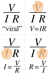
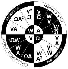
In circuit analysis, three equivalent expressions of Ohm's law are used interchangeably:

Each equation is quoted by some sources as the defining relationship of Ohm's law,[2][23][24] or all three are quoted,[25] or derived from a proportional form,[26] or even just the two that do not correspond to Ohm's original statement may sometimes be given.[27][28]
The interchangeability of the equation may be represented by a triangle, where V (voltage) is placed on the top section, the I (current) is placed to the left section, and the R (resistance) is placed to the right. The divider between the top and bottom sections indicates division (hence the division bar).
Resistive circuits edit
Resistors are circuit elements that impede the passage of electric charge in agreement with Ohm's law, and are designed to have a specific resistance value R. In schematic diagrams, a resistor is shown as a long rectangle or zig-zag symbol. An element (resistor or conductor) that behaves according to Ohm's law over some operating range is referred to as an ohmic device (or an ohmic resistor) because Ohm's law and a single value for the resistance suffice to describe the behavior of the device over that range.
Ohm's law holds for circuits containing only resistive elements (no capacitances or inductances) for all forms of driving voltage or current, regardless of whether the driving voltage or current is constant (DC) or time-varying such as AC. At any instant of time Ohm's law is valid for such circuits.
Resistors which are in series or in parallel may be grouped together into a single "equivalent resistance" in order to apply Ohm's law in analyzing the circuit.
Reactive circuits with time-varying signals edit
When reactive elements such as capacitors, inductors, or transmission lines are involved in a circuit to which AC or time-varying voltage or current is applied, the relationship between voltage and current becomes the solution to a differential equation, so Ohm's law (as defined above) does not directly apply since that form contains only resistances having value R, not complex impedances which may contain capacitance (C) or inductance (L).
Equations for time-invariant AC circuits take the same form as Ohm's law. However, the variables are generalized to complex numbers and the current and voltage waveforms are complex exponentials.[29]
In this approach, a voltage or current waveform takes the form Aest, where t is time, s is a complex parameter, and A is a complex scalar. In any linear time-invariant system, all of the currents and voltages can be expressed with the same s parameter as the input to the system, allowing the time-varying complex exponential term to be canceled out and the system described algebraically in terms of the complex scalars in the current and voltage waveforms.
The complex generalization of resistance is impedance, usually denoted Z; it can be shown that for an inductor,


We can now write,

This form of Ohm's law, with Z taking the place of R, generalizes the simpler form. When Z is complex, only the real part is responsible for dissipating heat.
In a general AC circuit, Z varies strongly with the frequency parameter s, and so also will the relationship between voltage and current.
For the common case of a steady sinusoid, the s parameter is taken to be , corresponding to a complex sinusoid . The real parts of such complex current and voltage waveforms describe the actual sinusoidal currents and voltages in a circuit, which can be in different phases due to the different complex scalars.


Linear approximations edit
Ohm's law is one of the basic equations used in the analysis of electrical circuits. It applies to both metal conductors and circuit components (resistors) specifically made for this behaviour. Both are ubiquitous in electrical engineering. Materials and components that obey Ohm's law are described as "ohmic"[30] which means they produce the same value for resistance (R = V/I) regardless of the value of V or I which is applied and whether the applied voltage or current is DC (direct current) of either positive or negative polarity or AC (alternating current).
In a true ohmic device, the same value of resistance will be calculated from R = V/I regardless of the value of the applied voltage V. That is, the ratio of V/I is constant, and when current is plotted as a function of voltage the curve is linear (a straight line). If voltage is forced to some value V, then that voltage V divided by measured current I will equal R. Or if the current is forced to some value I, then the measured voltage V divided by that current I is also R. Since the plot of I versus V is a straight line, then it is also true that for any set of two different voltages V1 and V2 applied across a given device of resistance R, producing currents I1 = V1/R and I2 = V2/R, that the ratio (V1 − V2)/(I1 − I2) is also a constant equal to R. The operator "delta" (Δ) is used to represent a difference in a quantity, so we can write ΔV = V1 − V2 and ΔI = I1 − I2. Summarizing, for any truly ohmic device having resistance R, V/I = ΔV/ΔI = R for any applied voltage or current or for the difference between any set of applied voltages or currents.
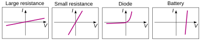
There are, however, components of electrical circuits which do not obey Ohm's law; that is, their relationship between current and voltage (their I–V curve) is nonlinear (or non-ohmic). An example is the p–n junction diode (curve at right). As seen in the figure, the current does not increase linearly with applied voltage for a diode. One can determine a value of current (I) for a given value of applied voltage (V) from the curve, but not from Ohm's law, since the value of "resistance" is not constant as a function of applied voltage. Further, the current only increases significantly if the applied voltage is positive, not negative. The ratio V/I for some point along the nonlinear curve is sometimes called the static, or chordal, or DC, resistance,[31][32] but as seen in the figure the value of total V over total I varies depending on the particular point along the nonlinear curve which is chosen. This means the "DC resistance" V/I at some point on the curve is not the same as what would be determined by applying an AC signal having peak amplitude ΔV volts or ΔI amps centered at that same point along the curve and measuring ΔV/ΔI. However, in some diode applications, the AC signal applied to the device is small and it is possible to analyze the circuit in terms of the dynamic, small-signal, or incremental resistance, defined as the one over the slope of the V–I curve at the average value (DC operating point) of the voltage (that is, one over the derivative of current with respect to voltage). For sufficiently small signals, the dynamic resistance allows the Ohm's law small signal resistance to be calculated as approximately one over the slope of a line drawn tangentially to the V–I curve at the DC operating point.[33]
Temperature effects edit
Ohm's law has sometimes been stated as, "for a conductor in a given state, the electromotive force is proportional to the current produced. "That is, that the resistance, the ratio of the applied electromotive force (or voltage) to the current, "does not vary with the current strength."The qualifier "in a given state" is usually interpreted as meaning "at a constant temperature," since the resistivity of materials is usually temperature dependent. Because the conduction of current is related to Joule heating of the conducting body, according to Joule's first law, the temperature of a conducting body may change when it carries a current. The dependence of resistance on temperature therefore makes resistance depend upon the current in a typical experimental setup, making the law in this form difficult to directly verify. Maxwell and others worked out several methods to test the law experimentally in 1876, controlling for heating effects.[34] Usually, the measurements of a sample resistance are carried out at low currents to prevent Joule heating. However, even a small current causes heating(cooling) at the first(second) sample contact due to the Peltier effect. The temperatures at the sample contacts become different, their difference is linear in current. The voltage drop across the circuit includes additionally the Seebeck thermoelectromotive force which again is again linear in current. As a result, there exists a thermal correction to the sample resistance even at negligibly small current.[35] The magnitude of the correction could be comparable with the sample resistance.[36]
Relation to heat conductions edit
Ohm's principle predicts the flow of electrical charge (i.e. current) in electrical conductors when subjected to the influence of voltage differences; Jean-Baptiste-Joseph Fourier's principle predicts the flow of heat in heat conductors when subjected to the influence of temperature differences.
The same equation describes both phenomena, the equation's variables taking on different meanings in the two cases. Specifically, solving a heat conduction (Fourier) problem with temperature (the driving "force") and flux of heat (the rate of flow of the driven "quantity", i.e. heat energy) variables also solves an analogous electrical conduction (Ohm) problem having electric potential (the driving "force") and electric current (the rate of flow of the driven "quantity", i.e. charge) variables.
The basis of Fourier's work was his clear conception and definition of thermal conductivity. He assumed that, all else being the same, the flux of heat is strictly proportional to the gradient of temperature. Although undoubtedly true for small temperature gradients, strictly proportional behavior will be lost when real materials (e.g. ones having a thermal conductivity that is a function of temperature) are subjected to large temperature gradients.
A similar assumption is made in the statement of Ohm's law: other things being alike, the strength of the current at each point is proportional to the gradient of electric potential. The accuracy of the assumption that flow is proportional to the gradient is more readily tested, using modern measurement methods, for the electrical case than for the heat case.
Other versions edit
Ohm's law, in the form above, is an extremely useful equation in the field of electrical/electronic engineering because it describes how voltage, current and resistance are interrelated on a "macroscopic" level, that is, commonly, as circuit elements in an electrical circuit. Physicists who study the electrical properties of matter at the microscopic level use a closely related and more general vector equation, sometimes also referred to as Ohm's law, having variables that are closely related to the V, I, and R scalar variables of Ohm's law, but which are each functions of position within the conductor. Physicists often use this continuum form of Ohm's Law:[37]

where E is the electric field vector with units of volts per meter (analogous to V of Ohm's law which has units of volts), J is the current density vector with units of amperes per unit area (analogous to I of Ohm's law which has units of amperes), and ρ "rho" is the resistivity with units of ohm·meters (analogous to R of Ohm's law which has units of ohms). The above equation is also written[38] as J = σE where σ "sigma" is the conductivity which is the reciprocal of ρ.

The voltage between two points is defined as:[39]


Since the E field is uniform in the direction of wire length, for a conductor having uniformly consistent resistivity ρ, the current density J will also be uniform in any cross-sectional area and oriented in the direction of wire length, so we may write:[40]

Substituting the above 2 results (for E and J respectively) into the continuum form shown at the beginning of this section:

The electrical resistance of a uniform conductor is given in terms of resistivity by:[40]

After substitution of R from the above equation into the equation preceding it, the continuum form of Ohm's law for a uniform field (and uniform current density) oriented along the length of the conductor reduces to the more familiar form:

A perfect crystal lattice, with low enough thermal motion and no deviations from periodic structure, would have no resistivity,[41] but a real metal has crystallographic defects, impurities, multiple isotopes, and thermal motion of the atoms. Electrons scatter from all of these, resulting in resistance to their flow.
The more complex generalized forms of Ohm's law are important to condensed matter physics, which studies the properties of matter and, in particular, its electronic structure. In broad terms, they fall under the topic of constitutive equations and the theory of transport coefficients.
Magnetic effects edit
If an external B-field is present and the conductor is not at rest but moving at velocity v, then an extra term must be added to account for the current induced by the Lorentz force on the charge carriers.

In the rest frame of the moving conductor this term drops out because v = 0. There is no contradiction because the electric field in the rest frame differs from the E-field in the lab frame: E′ = E + v × B. Electric and magnetic fields are relative, see Lorentz transformation.
If the current J is alternating because the applied voltage or E-field varies in time, then reactance must be added to resistance to account for self-inductance, see electrical impedance. The reactance may be strong if the frequency is high or the conductor is coiled.
Conductive fluids edit
In a conductive fluid, such as a plasma, there is a similar effect. Consider a fluid moving with the velocity in a magnetic field . The relative motion induces an electric field which exerts electric force on the charged particles giving rise to an electric current . The equation of motion for the electron gas, with a number density , is written as


where , and are the charge, mass and velocity of the electrons, respectively. Also, is the frequency of collisions of the electrons with ions which have a velocity field . Since, the electron has a very small mass compared with that of ions, we can ignore the left hand side of the above equation to write


where we have used the definition of the current density, and also put which is the electrical conductivity. This equation can also be equivalently written as


See also edit
References edit
- ^ Consoliver, Earl L. & Mitchell, Grover I. (1920). Automotive Ignition Systems. McGraw-Hill. p. 4.
- ^ a b Millikan, Robert A.; Bishop, E. S. (1917). Elements of Electricity. American Technical Society. p. 54.
- ^ Heaviside, Oliver (1894). Electrical Papers. Vol. 1. Macmillan and Co. p. 283. ISBN 978-0-8218-2840-3.
- ^ Young, Hugh; Freedman, Roger (2008). Sears and Zemansky's University Physics: With Modern Physics. Vol. 2 (12 ed.). Pearson. p. 853. ISBN 978-0-321-50121-9.
- ^ Darrigol, Olivier (8 June 2000). Electrodynamics from Ampère to Einstein. Clarendon Press. p. 70. ISBN 9780198505945..
- ^ Fleming, John Ambrose (1911). . In Chisholm, Hugh (ed.). Encyclopædia Britannica. Vol. 9 (11th ed.). Cambridge University Press. p. 182.
- ^ Bordeau, Sanford P. (1982). Volts to Hertz-- the Rise of Electricity: From the Compass to the Radio Through the Works of Sixteen Great Men of Science Whose Names are Used in Measuring Electricity and Magnetism. Burgess Publishing Company. pp. 86–107. ISBN 9780808749080.
- ^ Ronalds, B. F. (2016). Sir Francis Ronalds: Father of the Electric Telegraph. London: Imperial College Press. ISBN 978-1-78326-917-4.
- ^ Ronalds, B. F. (July 2016). "Francis Ronalds (1788–1873): The First Electrical Engineer?". Proceedings of the IEEE. 104 (7): 1489–1498. doi:10.1109/JPROC.2016.2571358. S2CID 20662894.
- ^ Ohm, G. S. (1827). Die galvanische Kette, mathematisch bearbeitet (PDF). Berlin: T. H. Riemann. Archived from the original (PDF) on 2009-03-26.
- ^ Davies, Brian (1980). "A web of naked fancies?". Physics Education. 15 (1): 57–61. Bibcode:1980PhyEd..15...57D. doi:10.1088/0031-9120/15/1/314. S2CID 250832899.
- ^ Hart, Ivor Blashka (1923). Makers of Science. London: Oxford University Press. p. 243. OL 6662681M..
- ^ Schnädelbach, Herbert (14 June 1984). Philosophy in Germany 1831-1933. Cambridge University Press. pp. 78–79. ISBN 9780521296465.
- ^ Taliaferro Preston (1855). Shaffner's Telegraph Companion: Devoted to the Science and Art of the Morse Telegraph. Vol. 2. Pudney & Russell.
- ^ Purcell, Edward M. (1985), Electricity and magnetism, Berkeley Physics Course, vol. 2 (2nd ed.), McGraw-Hill, p. 129, ISBN 978-0-07-004908-6
- ^ Griffiths, David J. (1999), Introduction to electrodynamics (3rd ed.), Prentice Hall, p. 289, ISBN 978-0-13-805326-0
- ^ Weber, B.; Mahapatra, S.; Ryu, H.; Lee, S.; Fuhrer, A.; Reusch, T. C. G.; Thompson, D. L.; Lee, W. C. T.; Klimeck, G.; Hollenberg, L. C. L.; Simmons, M. Y. (2012). "Ohm's Law Survives to the Atomic Scale". Science. 335 (6064): 64–67. Bibcode:2012Sci...335...64W. doi:10.1126/science.1214319. PMID 22223802. S2CID 10873901.
- ^ Drude, Paul (1900). "Zur Elektronentheorie der Metalle". Annalen der Physik. 306 (3): 566–613. Bibcode:1900AnP...306..566D. doi:10.1002/andp.19003060312.[dead link]
- ^ Drude, Paul (1900). "Zur Elektronentheorie der Metalle; II. Teil. Galvanomagnetische und thermomagnetische Effecte". Annalen der Physik. 308 (11): 369–402. Bibcode:1900AnP...308..369D. doi:10.1002/andp.19003081102.[dead link]
- ^ A. Akers; M. Gassman & R. Smith (2006). Hydraulic Power System Analysis. New York: Taylor & Francis. Chapter 13. ISBN 978-0-8247-9956-4.
- ^ A. Esposito, "A Simplified Method for Analyzing Circuits by Analogy", Machine Design, October 1969, pp. 173–177.
- ^ Guyton, Arthur; Hall, John (2006). "Chapter 14: Overview of the Circulation; Medical Physics of Pressure, Flow, and Resistance". In Gruliow, Rebecca (ed.). Textbook of Medical Physiology (11th ed.). Philadelphia, Pennsylvania: Elsevier Inc. p. 164. ISBN 978-0-7216-0240-0.
- ^ Nilsson, James William & Riedel, Susan A. (2008). Electric circuits. Prentice Hall. p. 29. ISBN 978-0-13-198925-2.
- ^ Halpern, Alvin M. & Erlbach, Erich (1998). Schaum's outline of theory and problems of beginning physics II. McGraw-Hill Professional. p. 140. ISBN 978-0-07-025707-8.
- ^ Patrick, Dale R. & Fardo, Stephen W. (1999). Understanding DC circuits. Newnes. p. 96. ISBN 978-0-7506-7110-1.
- ^ O'Conor Sloane, Thomas (1909). Elementary electrical calculations. D. Van Nostrand Co. p. 41.
R= Ohm's law proportional.
- ^ Cumming, Linnaeus (1902). Electricity treated experimentally for the use of schools and students. Longman's Green and Co. p. 220.
V=IR Ohm's law.
- ^ Stein, Benjamin (1997). Building technology (2nd ed.). John Wiley and Sons. p. 169. ISBN 978-0-471-59319-5.
- ^ Prasad, Rajendra (2006). Fundamentals of Electrical Engineering. Prentice-Hall of India. ISBN 978-81-203-2729-0.
- ^ Hughes, E, Electrical Technology, pp10, Longmans, 1969.
- ^ Brown, Forbes T. (2006). Engineering System Dynamics. CRC Press. p. 43. ISBN 978-0-8493-9648-9.
- ^ Kaiser, Kenneth L. (2004). Electromagnetic Compatibility Handbook. CRC Press. pp. 13–52. ISBN 978-0-8493-2087-3.
- ^ Horowitz, Paul; Hill, Winfield (1989). The Art of Electronics (2nd ed.). Cambridge University Press. p. 13. ISBN 978-0-521-37095-0.
- ^ Normal Lockyer, ed. (September 21, 1876). "Reports". Nature. 14 (360). Macmillan Journals Ltd: 451–459 [452]. Bibcode:1876Natur..14..451.. doi:10.1038/014451a0.
- ^ Kirby, C G M; Laubitz, M J (July 1973). "The Error Due to the Peltier Effect in Direct-Current Measurements of Resistance". Metrologia. 9 (3): 103–106. doi:10.1088/0026-1394/9/3/001. ISSN 0026-1394.
- ^ Cheremisin, M. V. (February 2001). "Peltier-effect-induced correction to ohmic resistance". Journal of Experimental and Theoretical Physics. 92 (2): 357–360. arXiv:physics/9908060. doi:10.1134/1.1354694. ISSN 1063-7761.
- ^ Lerner, Lawrence S. (1977). Physics for scientists and engineers. Jones & Bartlett. p. 736. ISBN 978-0-7637-0460-5.
- ^ Seymour J, Physical Electronics, Pitman, 1972, pp. 53–54
- ^ Lerner L, Physics for scientists and engineers, Jones & Bartlett, 1997, pp. 685–686
- ^ a b Lerner L, Physics for scientists and engineers, Jones & Bartlett, 1997, pp. 732–733
- ^ Seymour J, Physical Electronics, pp. 48–49, Pitman, 1972
Further reading edit
- Ohm's Law chapter from Lessons In Electric Circuits Vol 1 DC book and series.
- John C. Shedd and Mayo D. Hershey,"The History of Ohm's Law", Popular Science, December 1913, pp. 599–614, Bonnier Corporation ISSN 0161-7370, gives the history of Ohm's investigations, prior work, Ohm's false equation in the first paper, illustration of Ohm's experimental apparatus.
- Schagrin, Morton L. (1963). "Resistance to Ohm's Law". American Journal of Physics. 31 (7): 536–547. Bibcode:1963AmJPh..31..536S. doi:10.1119/1.1969620. S2CID 120421759. Explores the conceptual change underlying Ohm's experimental work.
- Kenneth L. Caneva, "Ohm, Georg Simon." Complete Dictionary of Scientific Biography. 2008
- s:Scientific Memoirs/2/The Galvanic Circuit investigated Mathematically, a translation of Ohm's original paper.
External links edit
- Ohms Law Calculator