


Summary
Orbit modeling is the process of creating mathematical models to simulate motion of a massive body as it moves in orbit around another massive body due to gravity. Other forces such as gravitational attraction from tertiary bodies, air resistance, solar pressure, or thrust from a propulsion system are typically modeled as secondary effects. Directly modeling an orbit can push the limits of machine precision due to the need to model small perturbations to very large orbits. Because of this, perturbation methods are often used to model the orbit in order to achieve better accuracy.
Background edit
The study of orbital motion and mathematical modeling of orbits began with the first attempts to predict planetary motions in the sky, although in ancient times the causes remained a mystery. Newton, at the time he formulated his laws of motion and of gravitation, applied them to the first analysis of perturbations,[1] recognizing the complex difficulties of their calculation.[1] Many of the great mathematicians since then have given attention to the various problems involved; throughout the 18th and 19th centuries there was demand for accurate tables of the position of the Moon and planets for purposes of navigation at sea.
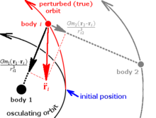
The complex motions of orbits can be broken down. The hypothetical motion that the body follows under the gravitational effect of one other body only is typically a conic section, and can be readily modeled with the methods of geometry. This is called a two-body problem, or an unperturbed Keplerian orbit. The differences between the Keplerian orbit and the actual motion of the body are caused by perturbations. These perturbations are caused by forces other than the gravitational effect between the primary and secondary body and must be modeled to create an accurate orbit simulation. Most orbit modeling approaches model the two-body problem and then add models of these perturbing forces and simulate these models over time. Perturbing forces may include gravitational attraction from other bodies besides the primary, solar wind, drag, magnetic fields, and propulsive forces.
Analytical solutions (mathematical expressions to predict the positions and motions at any future time) for simple two-body and three-body problems exist; none have been found for the n-body problem except for certain special cases. Even the two-body problem becomes insoluble if one of the bodies is irregular in shape.[2]
Due to the difficulty in finding analytic solutions to most problems of interest, computer modeling and simulation is typically used to analyze orbital motion. A wide variety of software is available to simulate orbits and trajectories of spacecraft.
Keplerian orbit model edit
In its simplest form, an orbit model can be created by assuming that only two bodies are involved, both behave as spherical point-masses, and that no other forces act on the bodies. For this case the model is simplified to a Kepler orbit.
Keplerian orbits follow conic sections. The mathematical model of the orbit which gives the distance between a central body and an orbiting body can be expressed as:

Where:
- is the distance
- is the semi-major axis, which defines the size of the orbit
- is the eccentricity, which defines the shape of the orbit
- is the true anomaly, which is the angle between the current position of the orbiting object and the location in the orbit at it is closest to the central body (called the periapsis)


Alternately, the equation can be expressed as:

Where is called the semi-latus rectum of the curve. This form of the equation is particularly useful when dealing with parabolic trajectories, for which the semi-major axis is infinite.

An alternate approach uses Isaac Newton's law of universal gravitation as defined below:

where:
- is the magnitude of the gravitational force between the two point masses
- is the gravitational constant
- is the mass of the first point mass
- is the mass of the second point mass
- is the distance between the two point masses


Making an additional assumption that the mass of the primary body is much greater than the mass of the secondary body and substituting in Newton's second law of motion, results in the following differential equation

Solving this differential equation results in Keplerian motion for an orbit. In practice, Keplerian orbits are typically only useful for first-order approximations, special cases, or as the base model for a perturbed orbit.
Orbit simulation methods edit
Orbit models are typically propagated in time and space using special perturbation methods. This is performed by first modeling the orbit as a Keplerian orbit. Then perturbations are added to the model to account for the various perturbations that affect the orbit.[1] Special perturbations can be applied to any problem in celestial mechanics, as it is not limited to cases where the perturbing forces are small.[2] Special perturbation methods are the basis of the most accurate machine-generated planetary ephemerides.[1] see, for instance, Jet Propulsion Laboratory Development Ephemeris
Cowell's method edit
Cowell's method is a special perturbation method;[3] mathematically, for mutually interacting bodies, Newtonian forces on body from the other bodies are simply summed thus,


where
- is the acceleration vector of body
- is the gravitational constant
- is the mass of body
- and are the position vectors of objects and
- is the distance from object to object


with all vectors being referred to the barycenter of the system. This equation is resolved into components in , , and these are integrated numerically to form the new velocity and position vectors as the simulation moves forward in time. The advantage of Cowell's method is ease of application and programming. A disadvantage is that when perturbations become large in magnitude (as when an object makes a close approach to another) the errors of the method also become large.[4] Another disadvantage is that in systems with a dominant central body, such as the Sun, it is necessary to carry many significant digits in the arithmetic because of the large difference in the forces of the central body and the perturbing bodies.[5]


Encke's method edit

Encke's method begins with the osculating orbit as a reference and integrates numerically to solve for the variation from the reference as a function of time.[6] Its advantages are that perturbations are generally small in magnitude, so the integration can proceed in larger steps (with resulting lesser errors), and the method is much less affected by extreme perturbations than Cowell's method. Its disadvantage is complexity; it cannot be used indefinitely without occasionally updating the osculating orbit and continuing from there, a process known as rectification.[4] [7]
Letting be the radius vector of the osculating orbit, the radius vector of the perturbed orbit, and the variation from the osculating orbit,


-
(1)

-
(2)

and are just the equations of motion of and ,


-
for the perturbed orbit and
(3)

-
for the unperturbed orbit,
(4)

where is the gravitational parameter with and the masses of the central body and the perturbed body, is the perturbing acceleration, and and are the magnitudes of and .


Substituting from equations (3) and (4) into equation (2),
-
(5)

which, in theory, could be integrated twice to find . Since the osculating orbit is easily calculated by two-body methods, and are accounted for and can be solved. In practice, the quantity in the brackets, , is the difference of two nearly equal vectors, and further manipulation is necessary to avoid the need for extra significant digits.[8][9]

Sperling–Burdet method edit
In 1991 Victor R. Bond and Michael F. Fraietta created an efficient and highly accurate method for solving the two-body perturbed problem.[10] This method uses the linearized and regularized differential equations of motion derived by Hans Sperling and a perturbation theory based on these equations developed by C.A. Burdet in the year 1864. In 1973, Bond and Hanssen improved Burdet's set of differential equations by using the total energy of the perturbed system as a parameter instead of the two-body energy and by reducing the number of elements to 13. In 1989 Bond and Gottlieb embedded the Jacobian integral, which is a constant when the potential function is explicitly dependent upon time as well as position in the Newtonian equations. The Jacobian constant was used as an element to replace the total energy in a reformulation of the differential equations of motion. In this process, another element which is proportional to a component of the angular momentum is introduced. This brought the total number of elements back to 14. In 1991, Bond and Fraietta made further revisions by replacing the Laplace vector with another vector integral as well as another scalar integral which removed small secular terms which appeared in the differential equations for some of the elements.[11]
The Sperling–Burdet method is executed in a 5 step process as follows:[11]
- Step 1: Initialization
- Given an initial position, , an initial velocity, , and an initial time, , the following variables are initialized:
- Perturbations due to perturbing masses, defined as and , are evaluated
- Perturbations due to other accelerations, defined as , are evaluated
- Step 2: Transform elements to coordinates
- where are Stumpff functions
- Step 3: Evaluate differential equations for the elements
- Step 4: Integration
- Here the differential equations are integrated over a period to obtain the element value at
- Step 5: Advance
- Set and return to step 2 until simulation stopping conditions are met.


![{\displaystyle {\Bigg [}{\partial {V} \over {\partial {\mathbf {r} }}}{\Bigg ]}_{0}}](https://wikimedia.org/api/rest_v1/media/math/render/svg/612f025d580a4b1bf33508dbc3d44829e64e0717)


![{\displaystyle {\boldsymbol {\alpha }}'=-\mathbf {Q} sc_{1}-\mu {\boldsymbol {\epsilon }}'s^{2}c_{2}-\alpha '_{J}{\big [}{\boldsymbol {\alpha }}s^{2}c_{2}+2{\boldsymbol {\beta }}s^{3}{\bar {c}}_{3}+{\frac {1}{2}}{\boldsymbol {\delta }}s^{4}c_{2}^{2}{\big ]}}](https://wikimedia.org/api/rest_v1/media/math/render/svg/6f9ccac2afa1c8ff5a9c69faf3008d39d0a7ae22)
![{\displaystyle {\boldsymbol {\beta }}'=\mathbf {Q} c_{0}+\mu {\boldsymbol {\epsilon }}'sc_{1}+\alpha '_{J}{\big [}{\boldsymbol {\alpha }}sc_{1}+{\boldsymbol {\beta }}s^{2}{\bar {c}}_{2}-{\boldsymbol {\delta }}s^{3}(2{\bar {c}}_{3}-c_{1}c_{2}){\big ]}}](https://wikimedia.org/api/rest_v1/media/math/render/svg/9dcee48680100c98df2619a057fb7943551c61a2)
![{\displaystyle {\boldsymbol {\delta }}'=\mathbf {Q} \alpha _{J}sc_{1}-\mu {\boldsymbol {\epsilon }}'c_{0}+\alpha '_{J}{\big [}-{\boldsymbol {\alpha }}c_{0}+2\alpha _{J}{\boldsymbol {\beta }}s^{3}{\bar {c}}_{3}+{\frac {1}{2}}{\boldsymbol {\delta }}\alpha _{J}s^{4}c_{2}^{2}{\big ]}}](https://wikimedia.org/api/rest_v1/media/math/render/svg/93985eb591350494c7f2233e6a42546e1bb6cdfc)

![{\displaystyle a'=-{\frac {1}{r}}\mathbf {r} \cdot \mathbf {Q} sc_{1}-\alpha _{J}'{\big [}as^{2}c_{2}+2bs^{3}{\bar {c}}_{3}+{\frac {1}{2}}\gamma s^{4}c_{2}^{2}{\big ]}}](https://wikimedia.org/api/rest_v1/media/math/render/svg/4ee754eeec77a59bce529490884dc4f26522fb3e)
![{\displaystyle b'={\frac {1}{r}}\mathbf {r} \cdot \mathbf {Q} c_{0}+\alpha _{J}'{\big [}asc_{1}+bs^{2}{\bar {c}}_{2}-\gamma s^{3}(2{\bar {c}}_{3}-c_{1}c_{2}){\big ]}}](https://wikimedia.org/api/rest_v1/media/math/render/svg/433f2aafc73516bb710427d409458265912631a3)
![{\displaystyle \gamma '=-{\frac {1}{r}}\mathbf {r} \cdot \mathbf {Q} \alpha _{J}sc_{1}+\alpha _{J}'{\big [}-ac_{0}+2b\alpha _{J}s^{3}{\bar {c}}_{3}+{\frac {1}{2}}\gamma \alpha _{J}s^{4}c_{2}^{2}{\big ]}}](https://wikimedia.org/api/rest_v1/media/math/render/svg/8af2838185f2b6697f564fb381762f7db2fe0116)
![{\displaystyle \tau '={\frac {1}{r}}\mathbf {r} \cdot \mathbf {Q} s^{2}c_{2}+\alpha _{J}'{\big [}as^{3}c_{3}+{\frac {1}{2}}bs^{4}c_{2}^{2}-2\gamma s^{5}(c_{5}-4{\bar {c}}_{5}){\big ]}}](https://wikimedia.org/api/rest_v1/media/math/render/svg/0c41f15f1e244d420815999f192d808609cbd573)


Perturbations edit
Perturbing forces cause orbits to become perturbed from a perfect Keplerian orbit. Models for each of these forces are created and executed during the orbit simulation so their effects on the orbit can be determined.
Non-spherical gravity edit
The Earth is not a perfect sphere nor is mass evenly distributed within the Earth. This results in the point-mass gravity model being inaccurate for orbits around the Earth, particularly Low Earth orbits. To account for variations in gravitational potential around the surface of the Earth, the gravitational field of the Earth is modeled with spherical harmonics[12] which are expressed through the equation:

where
- is the gravitational parameter defined as the product of G, the universal gravitational constant, and the mass of the primary body.
- is the unit vector defining the distance between the primary and secondary bodies, with being the magnitude of the distance.
- represents the contribution to of the spherical harmonic of degree n and order m, which is defined as:[12]


![{\displaystyle {\begin{aligned}\mathbf {f} _{n,m}&={\frac {\mu R_{O}^{2}}{R^{n+m+1}}}\left({\frac {C_{n,m}{\mathcal {C}}_{m}+S_{n,m}{\mathcal {S}}_{m}}{R}}(A_{n,m+1}\mathbf {\hat {e}} _{3}-\left(s_{\lambda }A_{n,m+1}+(n+m+1)A_{n,m}\right)\mathbf {\hat {r}} \right)\\[10pt]&{}\quad {}+mA_{n,m}((C_{n,m}{\mathcal {C}}_{m-1}+S_{n,m}{\mathcal {S}}_{m-1})\mathbf {\hat {e}} _{1}+(S_{n,m}{\mathcal {C}}_{m-1}-C_{n,m}{\mathcal {S}}_{m-1})\mathbf {\hat {e}} _{2}))\end{aligned}}}](https://wikimedia.org/api/rest_v1/media/math/render/svg/76b77d819bc184cb3c4e167b9775f7b12d0e1cfb)
where:
- is the mean equatorial radius of the primary body.
- is the magnitude of the position vector from the center of the primary body to the center of the secondary body.
- and are gravitational coefficients of degree n and order m. These are typically found through gravimetry measurements.
- The unit vectors define a coordinate system fixed on the primary body. For the Earth, lies in the equatorial plane parallel to a line intersecting Earth's geometric center and the Greenwich meridian, points in the direction of the North polar axis, and
- is referred to as a derived Legendre polynomial of degree n and order m. They are solved through the recurrence relation:
- is sine of the geographic latitude of the secondary body, which is .
- are defined with the following recurrence relation and initial conditions:


When modeling perturbations of an orbit around a primary body only the sum of the terms need to be included in the perturbation since the point-mass gravity model is accounted for in the term

Third-body perturbations edit
Gravitational forces from third bodies can cause perturbations to an orbit. For example, the Sun and Moon cause perturbations to Orbits around the Earth.[13] These forces are modeled in the same way that gravity is modeled for the primary body by means of direct gravitational N-body simulations. Typically, only a spherical point-mass gravity model is used for modeling effects from these third bodies.[14] Some special cases of third-body perturbations have approximate analytic solutions. For example, perturbations for the right ascension of the ascending node and argument of perigee for a circular Earth orbit are:[13]
- where:
- is the change to the right ascension of the ascending node in degrees per day.
- is the change to the argument of perigee in degrees per day.
- is the orbital inclination.
- is the number of orbital revolutions per day.


Solar radiation edit
Solar radiation pressure causes perturbations to orbits. The magnitude of acceleration it imparts to a spacecraft in Earth orbit is modeled using the equation below:[13]

where:
- is the magnitude of acceleration in meters per second-squared.
- is the cross-sectional area exposed to the Sun in meters-squared.
- is the spacecraft mass in kilograms.
- is the reflection factor which depends on material properties. for absorption, for specular reflection, and for diffuse reflection.


For orbits around the Earth, solar radiation pressure becomes a stronger force than drag above 800 km altitude.[13]
Propulsion edit
There are many different types of spacecraft propulsion. Rocket engines are one of the most widely used. The force of a rocket engine is modeled by the equation:[15]

where: = exhaust gas mass flow = effective exhaust velocity = actual jet velocity at nozzle exit plane = flow area at nozzle exit plane (or the plane where the jet leaves the nozzle if separated flow) = static pressure at nozzle exit plane = ambient (or atmospheric) pressure


Another possible method is a solar sail. Solar sails use radiation pressure in a way to achieve a desired propulsive force.[16] The perturbation model due to the solar wind can be used as a model of propulsive force from a solar sail.
Drag edit
The primary non-gravitational force acting on satellites in low Earth orbit is atmospheric drag.[13] Drag will act in opposition to the direction of velocity and remove energy from an orbit. The force due to drag is modeled by the following equation:

where
- is the force of drag,
- is the density of the fluid,[17]
- is the velocity of the object relative to the fluid,
- is the drag coefficient (a dimensionless parameter, e.g. 2 to 4 for most satellites[13])
- is the reference area.


Orbits with an altitude below 120 km generally have such high drag that the orbits decay too rapidly to give a satellite a sufficient lifetime to accomplish any practical mission. On the other hand, orbits with an altitude above 600 km have relatively small drag so that the orbit decays slow enough that it has no real impact on the satellite over its useful life.[13] Density of air can vary significantly in the thermosphere where most low Earth orbiting satellites reside. The variation is primarily due to solar activity, and thus solar activity can greatly influence the force of drag on a spacecraft and complicate long-term orbit simulation.[13]
Magnetic fields edit
Magnetic fields can play a significant role as a source of orbit perturbation as was seen in the Long Duration Exposure Facility.[12] Like gravity, the magnetic field of the Earth can be expressed through spherical harmonics as shown below:[12]

where
- is the magnetic field vector at a point above the Earth's surface.
- represents the contribution to of the spherical harmonic of degree n and order m, defined as:[12]


![{\displaystyle {\begin{aligned}\mathbf {B} _{n,m}={}&{\frac {K_{n,m}a^{n+2}}{R^{n+m+1}}}\left[{\frac {g_{n,m}{\mathcal {C}}_{m}+h_{n,m}{\mathcal {S}}_{m}}{R}}((s_{\lambda }A_{n,m+1}+(n+m+1)A_{n,m})\mathbf {\hat {r}} )-A_{n,m+1}\mathbf {\hat {e}} _{3}\right]\\[10pt]&{}-mA_{n,m}((g_{n,m}{\mathcal {C}}_{m-1}+h_{n,m}{\mathcal {S}}_{m-1})\mathbf {\hat {e}} _{1}+(h_{n,m}{\mathcal {C}}_{m-1}-g_{n,m}{\mathcal {S}}_{m-1})\mathbf {\hat {e}} _{2}))\end{aligned}}}](https://wikimedia.org/api/rest_v1/media/math/render/svg/da4332b01a6ef5c1675f0821a6f3fa44eaa699bf)
where:
- is the mean equatorial radius of the primary body.
- is the magnitude of the position vector from the center of the primary body to the center of the secondary body.
- is a unit vector in the direction of the secondary body with its origin at the center of the primary body.
- and are Gauss coefficients of degree n and order m. These are typically found through magnetic field measurements.
- The unit vectors define a coordinate system fixed on the primary body. For the Earth, lies in the equatorial plane parallel to a line intersecting Earth's geometric center and the Greenwich meridian, points in the direction of the North polar axis, and
- is referred to as a derived Legendre polynomial of degree n and order m. They are solved through the recurrence relation:
- is defined as: 1 if m = 0, for and , and for and
- is sine of the geographic latitude of the secondary body, which is .
- are defined with the following recurrence relation and initial conditions:


![{\displaystyle {\big [}{\frac {n-m}{n+m}}{\big ]}^{0.5}K_{n-1,m}}](https://wikimedia.org/api/rest_v1/media/math/render/svg/749b20930188e56320936df0e7700d81fd2e6b32)

![{\displaystyle m=[1\ldots \infty ]}](https://wikimedia.org/api/rest_v1/media/math/render/svg/62bd1323df293b9995b0034881c1a1f2280bfd82)
![{\displaystyle [(n+m)(n-m+1)]^{-0.5}K_{n,m-1}}](https://wikimedia.org/api/rest_v1/media/math/render/svg/4062cf10e251e74c0aabd08f6ec3811c8d5d58ed)

![{\displaystyle m=[2\ldots \infty ]}](https://wikimedia.org/api/rest_v1/media/math/render/svg/5b211a8fb79a80430ea446e5a380bd1151be0974)
See also edit
Notes and references edit
- ^ a b c d Moulton, Forest Ray (1914). "Chapter IX". An Introduction to Celestial Mechanics (Second Revised ed.). Macmillan. ISBN 9780598943972.
- ^ a b Roy, A.E. (1988). "Chapters 6 and 7". Orbital Motion (third ed.). Institute of Physics Publishing. ISBN 978-0-85274-229-7.
- ^ So named for Philip H. Cowell, who, with A.C.D. Cromellin, used a similar method to predict the return of Halley's comet. Brouwer, Dirk; Clemence, Gerald M. (1961). Methods of Celestial Mechanics. Academic Press, New York and London. p. 186.
- ^ a b Danby, J.M.A. (1988). "Chapter 11". Fundamentals of Celestial Mechanics (second ed.). Willmann-Bell, Inc. ISBN 978-0-943396-20-0.
- ^ Herget, Paul (1948). The Computation of Orbits. privately published by the author. p. 91 ff.
- ^ So named for Johann Franz Encke; Battin, Richard H. (1999). An Introduction to the Mathematics and Methods of Astrodynamics, Revised Edition. American Institute of Aeronautics and Astronautics, Inc. p. 448. ISBN 978-1-56347-342-5.
- ^ Battin (1999), sec. 10.2.
- ^ Bate, Mueller, White (1971), sec. 9.3.
- ^ Roy (1988), sec. 7.4.
- ^ Peláez, Jesús; José Manuel Hedo; Pedro Rodríguez de Andrés (13 October 2006). "A special perturbation method in orbital dynamics". Celest. Mech. Dyn. Astron. 97 (2): 131–150. Bibcode:2007CeMDA..97..131P. doi:10.1007/s10569-006-9056-3. S2CID 35352081.
- ^ a b Bond, Victor; Michael F. Fraietta (1991). "Elimination Of Secular Terms From The Differential Equations For The Elements of Perturbed Two-Body Motion". Flight Mechanics and Estimation Theory Symposium.
- ^ a b c d e Roithmayr, Carlos (March 2004). "Contributions of Spherical Harmonics to Magnetic and Gravitational Fields". Nasa/Tm–2004–213007.
- ^ a b c d e f g h Larson, Wiley (1999). Space Mission Analysis and Design. California: Microcosm Press. ISBN 978-1-881883-10-4.
- ^ Delgado, Manuel. "Third Body Perturbation Modeling the Space Environment" (PDF). European Masters in Aeronautics and Space. Universidad Polit ´ecnica de Madrid. Archived from the original (PDF) on 18 February 2015. Retrieved 27 November 2012.
- ^ George P. Sutton & Oscar Biblarz (2001). Rocket Propulsion Elements (7th ed.). Wiley Interscience. ISBN 978-0-471-32642-7. See Equation 2-14.
- ^ "MESSENGER Sails on Sun's Fire for Second Flyby of Mercury". 2008-09-05. Archived from the original on 2013-05-14.
On September 4, the MESSENGER team announced that it would not need to implement a scheduled maneuver to adjust the probe's trajectory. This is the fourth time this year that such a maneuver has been called off. The reason? A recently implemented navigational technique that makes use of solar-radiation pressure (SRP) to guide the probe has been extremely successful at maintaining MESSENGER on a trajectory that will carry it over the cratered surface of Mercury for a second time on October 6.
- ^ Note that for the Earth's atmosphere, the air density can be found using the barometric formula. It is 1.293 kg/m3 at 0 °C and 1 atmosphere.
External links edit
- [1] Gravity maps of the Earth