


Summary
In geometry, the Peano curve is the first example of a space-filling curve to be discovered, by Giuseppe Peano in 1890.[1] Peano's curve is a surjective, continuous function from the unit interval onto the unit square, however it is not injective. Peano was motivated by an earlier result of Georg Cantor that these two sets have the same cardinality. Because of this example, some authors use the phrase "Peano curve" to refer more generally to any space-filling curve.[2]


Construction edit
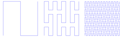
Peano's curve may be constructed by a sequence of steps, where the ith step constructs a set Si of squares, and a sequence Pi of the centers of the squares, from the set and sequence constructed in the previous step. As a base case, S0 consists of the single unit square, and P0 is the one-element sequence consisting of its center point.
In step i, each square s of Si − 1 is partitioned into nine smaller equal squares, and its center point c is replaced by a contiguous subsequence of the centers of these nine smaller squares. This subsequence is formed by grouping the nine smaller squares into three columns, ordering the centers contiguously within each column, and then ordering the columns from one side of the square to the other, in such a way that the distance between each consecutive pair of points in the subsequence equals the side length of the small squares. There are four such orderings possible:
- Left three centers bottom to top, middle three centers top to bottom, and right three centers bottom to top
- Right three centers bottom to top, middle three centers top to bottom, and left three centers bottom to top
- Left three centers top to bottom, middle three centers bottom to top, and right three centers top to bottom
- Right three centers top to bottom, middle three centers bottom to top, and left three centers top to bottom
Among these four orderings, the one for s is chosen in such a way that the distance between the first point of the ordering and its predecessor in Pi also equals the side length of the small squares. If c was the first point in its ordering, then the first of these four orderings is chosen for the nine centers that replace c.[3]
The Peano curve itself is the limit of the curves through the sequences of square centers, as i goes to infinity.
Variants edit

In the definition of the Peano curve, it is possible to perform some or all of the steps by making the centers of each row of three squares be contiguous, rather than the centers of each column of squares. These choices lead to many different variants of the Peano curve.[3]
A "multiple radix" variant of this curve with different numbers of subdivisions in different directions can be used to fill rectangles of arbitrary shapes.[4]
The Hilbert curve is a simpler variant of the same idea, based on subdividing squares into four equal smaller squares instead of into nine equal smaller squares.
References edit
- ^ Peano, G. (1890), "Sur une courbe, qui remplit toute une aire plane", Mathematische Annalen, 36 (1): 157–160, doi:10.1007/BF01199438.
- ^ Gugenheimer, Heinrich Walter (1963), Differential Geometry, Courier Dover Publications, p. 3, ISBN 9780486157207.
- ^ a b Bader, Michael (2013), "2.4 Peano curve", Space-Filling Curves, Texts in Computational Science and Engineering, vol. 9, Springer, pp. 25–27, doi:10.1007/978-3-642-31046-1_2, ISBN 9783642310461.
- ^ Cole, A. J. (September 1991), "Halftoning without dither or edge enhancement", The Visual Computer, 7 (5): 235–238, doi:10.1007/BF01905689