


Summary
In physics, the Poynting vector (or Umov–Poynting vector) represents the directional energy flux (the energy transfer per unit area, per unit time) or power flow of an electromagnetic field. The SI unit of the Poynting vector is the watt per square metre (W/m2); kg/s3 in base SI units. It is named after its discoverer John Henry Poynting who first derived it in 1884.[1]: 132 Nikolay Umov is also credited with formulating the concept.[2] Oliver Heaviside also discovered it independently in the more general form that recognises the freedom of adding the curl of an arbitrary vector field to the definition.[3] The Poynting vector is used throughout electromagnetics in conjunction with Poynting's theorem, the continuity equation expressing conservation of electromagnetic energy, to calculate the power flow in electromagnetic fields.
Definition edit
In Poynting's original paper and in most textbooks, the Poynting vector is defined as the cross product[4][5][6]


- E is the electric field vector;
- H is the magnetic field's auxiliary field vector or magnetizing field.
This expression is often called the Abraham form and is the most widely used.[7] The Poynting vector is usually denoted by S or N.
In simple terms, the Poynting vector S depicts the direction and rate of transfer of energy, that is power, due to electromagnetic fields in a region of space that may or may not be empty. More rigorously, it is the quantity that must be used to make Poynting's theorem valid. Poynting's theorem essentially says that the difference between the electromagnetic energy entering a region and the electromagnetic energy leaving a region must equal the energy converted or dissipated in that region, that is, turned into a different form of energy (often heat). So if one accepts the validity of the Poynting vector description of electromagnetic energy transfer, then Poynting's theorem is simply a statement of the conservation of energy.
If electromagnetic energy is not gained from or lost to other forms of energy within some region (e.g., mechanical energy, or heat), then electromagnetic energy is locally conserved within that region, yielding a continuity equation as a special case of Poynting's theorem:


Example: Power flow in a coaxial cable edit
Although problems in electromagnetics with arbitrary geometries are notoriously difficult to solve, we can find a relatively simple solution in the case of power transmission through a section of coaxial cable analyzed in cylindrical coordinates as depicted in the accompanying diagram. We can take advantage of the model's symmetry: no dependence on θ (circular symmetry) nor on Z (position along the cable). The model (and solution) can be considered simply as a DC circuit with no time dependence, but the following solution applies equally well to the transmission of radio frequency power, as long as we are considering an instant of time (during which the voltage and current don't change), and over a sufficiently short segment of cable (much smaller than a wavelength, so that these quantities are not dependent on Z). The coaxial cable is specified as having an inner conductor of radius R1 and an outer conductor whose inner radius is R2 (its thickness beyond R2 doesn't affect the following analysis). In between R1 and R2 the cable contains an ideal dielectric material of relative permittivity εr and we assume conductors that are non-magnetic (so μ = μ0) and lossless (perfect conductors), all of which are good approximations to real-world coaxial cable in typical situations.


The center conductor is held at voltage V and draws a current I toward the right, so we expect a total power flow of P = V · I according to basic laws of electricity. By evaluating the Poynting vector, however, we are able to identify the profile of power flow in terms of the electric and magnetic fields inside the coaxial cable. The electric fields are of course zero inside of each conductor, but in between the conductors ( ) symmetry dictates that they are strictly in the radial direction and it can be shown (using Gauss's law) that they must obey the following form:


The magnetic field, again by symmetry, can only be non-zero in the θ direction, that is, a vector field looping around the center conductor at every radius between R1 and R2. Inside the conductors themselves the magnetic field may or may not be zero, but this is of no concern since the Poynting vector in these regions is zero due to the electric field's being zero. Outside the entire coaxial cable, the magnetic field is identically zero since paths in this region enclose a net current of zero (+I in the center conductor and −I in the outer conductor), and again the electric field is zero there anyway. Using Ampère's law in the region from R1 to R2, which encloses the current +I in the center conductor but with no contribution from the current in the outer conductor, we find at radius r:


Substituting the earlier solution for the constant W we find:

Other similar examples in which the P = V · I result can be analytically calculated are: the parallel-plate transmission line,[8] using Cartesian coordinates, and the two-wire transmission line,[9] using bipolar cylindrical coordinates.
Other forms edit
In the "microscopic" version of Maxwell's equations, this definition must be replaced by a definition in terms of the electric field E and the magnetic flux density B (described later in the article).
It is also possible to combine the electric displacement field D with the magnetic flux B to get the Minkowski form of the Poynting vector, or use D and H to construct yet another version. The choice has been controversial: Pfeifer et al.[10] summarize and to a certain extent resolve the century-long dispute between proponents of the Abraham and Minkowski forms (see Abraham–Minkowski controversy).
The Poynting vector represents the particular case of an energy flux vector for electromagnetic energy. However, any type of energy has its direction of movement in space, as well as its density, so energy flux vectors can be defined for other types of energy as well, e.g., for mechanical energy. The Umov–Poynting vector[11] discovered by Nikolay Umov in 1874 describes energy flux in liquid and elastic media in a completely generalized view.
Interpretation edit
The Poynting vector appears in Poynting's theorem (see that article for the derivation), an energy-conservation law:


- E is the electric field;
- D is the electric displacement field;
- B is the magnetic flux density;
- H is the magnetizing field.[12]: 258–260
The first term in the right-hand side represents the electromagnetic energy flow into a small volume, while the second term subtracts the work done by the field on free electrical currents, which thereby exits from electromagnetic energy as dissipation, heat, etc. In this definition, bound electrical currents are not included in this term and instead contribute to S and u.
For linear, nondispersive and isotropic (for simplicity) materials, the constitutive relations can be written as

- ε is the permittivity of the material;
- μ is the permeability of the material.[12]: 258–260
Here ε and μ are scalar, real-valued constants independent of position, direction, and frequency.
In principle, this limits Poynting's theorem in this form to fields in vacuum and nondispersive[clarification needed] linear materials. A generalization to dispersive materials is possible under certain circumstances at the cost of additional terms.[12]: 262–264
One consequence of the Poynting formula is that for the electromagnetic field to do work, both magnetic and electric fields must be present. The magnetic field alone or the electric field alone cannot do any work.[13]
Plane waves edit
In a propagating electromagnetic plane wave in an isotropic lossless medium, the instantaneous Poynting vector always points in the direction of propagation while rapidly oscillating in magnitude. This can be simply seen given that in a plane wave, the magnitude of the magnetic field H(r,t) is given by the magnitude of the electric field vector E(r,t) divided by η, the intrinsic impedance of the transmission medium:


Finding the time-averaged power in the plane wave then requires averaging over the wave period (the inverse frequency of the wave):


In optics, the value of radiated flux crossing a surface, thus the average Poynting vector component in the direction normal to that surface, is technically known as the irradiance, more often simply referred to as the intensity (a somewhat ambiguous term).
Formulation in terms of microscopic fields edit
The "microscopic" (differential) version of Maxwell's equations admits only the fundamental fields E and B, without a built-in model of material media. Only the vacuum permittivity and permeability are used, and there is no D or H. When this model is used, the Poynting vector is defined as

- μ0 is the vacuum permeability;
- E is the electric field vector;
- B is the magnetic flux.
This is actually the general expression of the Poynting vector[dubious ].[14] The corresponding form of Poynting's theorem is


The two alternative definitions of the Poynting vector are equal in vacuum or in non-magnetic materials, where B = μ0H. In all other cases, they differ in that S = (1/μ0) E × B and the corresponding u are purely radiative, since the dissipation term −J ⋅ E covers the total current, while the E × H definition has contributions from bound currents which are then excluded from the dissipation term.[15]
Since only the microscopic fields E and B occur in the derivation of S = (1/μ0) E × B and the energy density, assumptions about any material present are avoided. The Poynting vector and theorem and expression for energy density are universally valid in vacuum and all materials.[15]
Time-averaged Poynting vector edit
The above form for the Poynting vector represents the instantaneous power flow due to instantaneous electric and magnetic fields. More commonly, problems in electromagnetics are solved in terms of sinusoidally varying fields at a specified frequency. The results can then be applied more generally, for instance, by representing incoherent radiation as a superposition of such waves at different frequencies and with fluctuating amplitudes.
We would thus not be considering the instantaneous E(t) and H(t) used above, but rather a complex (vector) amplitude for each which describes a coherent wave's phase (as well as amplitude) using phasor notation. These complex amplitude vectors are not functions of time, as they are understood to refer to oscillations over all time. A phasor such as Em is understood to signify a sinusoidally varying field whose instantaneous amplitude E(t) follows the real part of Em ejωt where ω is the (radian) frequency of the sinusoidal wave being considered.
In the time domain, it will be seen that the instantaneous power flow will be fluctuating at a frequency of 2ω. But what is normally of interest is the average power flow in which those fluctuations are not considered. In the math below, this is accomplished by integrating over a full cycle T = 2π / ω. The following quantity, still referred to as a "Poynting vector", is expressed directly in terms of the phasors as:

where ∗ denotes the complex conjugate. The time-averaged power flow (according to the instantaneous Poynting vector averaged over a full cycle, for instance) is then given by the real part of Sm. The imaginary part is usually ignored, however, it signifies "reactive power" such as the interference due to a standing wave or the near field of an antenna. In a single electromagnetic plane wave (rather than a standing wave which can be described as two such waves travelling in opposite directions), E and H are exactly in phase, so Sm is simply a real number according to the above definition.
The equivalence of Re(Sm) to the time-average of the instantaneous Poynting vector S can be shown as follows.

The average of the instantaneous Poynting vector S over time is given by:
![{\displaystyle \langle \mathbf {S} \rangle ={\frac {1}{T}}\int _{0}^{T}\mathbf {S} (t)\,dt={\frac {1}{T}}\int _{0}^{T}\!\left[{\tfrac {1}{2}}\operatorname {Re} \!\left(\mathbf {E} _{\mathrm {m} }\times \mathbf {H} _{\mathrm {m} }^{*}\right)+{\tfrac {1}{2}}\operatorname {Re} \!\left({\mathbf {E} _{\mathrm {m} }}\times {\mathbf {H} _{\mathrm {m} }}e^{2j\omega t}\right)\right]dt.}](https://wikimedia.org/api/rest_v1/media/math/render/svg/9d6783ee9e038080c9c4768c26588ac2a5f25e9f)
The second term is the double-frequency component having an average value of zero, so we find:

According to some conventions, the factor of 1/2 in the above definition may be left out. Multiplication by 1/2 is required to properly describe the power flow since the magnitudes of Em and Hm refer to the peak fields of the oscillating quantities. If rather the fields are described in terms of their root mean square (RMS) values (which are each smaller by the factor ), then the correct average power flow is obtained without multiplication by 1/2.

Resistive dissipation edit
If a conductor has significant resistance, then, near the surface of that conductor, the Poynting vector would be tilted toward and impinge upon the conductor.[9]: figs.7,8 Once the Poynting vector enters the conductor, it is bent to a direction that is almost perpendicular to the surface.[16]: 61 This is a consequence of Snell's law and the very slow speed of light inside a conductor. The definition and computation of the speed of light in a conductor can be given.[17]: 402 Inside the conductor, the Poynting vector represents energy flow from the electromagnetic field into the wire, producing resistive Joule heating in the wire. For a derivation that starts with Snell's law see Reitz page 454.[18]: 454
Radiation pressure edit
The density of the linear momentum of the electromagnetic field is S/c2 where S is the magnitude of the Poynting vector and c is the speed of light in free space. The radiation pressure exerted by an electromagnetic wave on the surface of a target is given by

Uniqueness of the Poynting vector edit
The Poynting vector occurs in Poynting's theorem only through its divergence ∇ ⋅ S, that is, it is only required that the surface integral of the Poynting vector around a closed surface describe the net flow of electromagnetic energy into or out of the enclosed volume. This means that adding a solenoidal vector field (one with zero divergence) to S will result in another field that satisfies this required property of a Poynting vector field according to Poynting's theorem. Since the divergence of any curl is zero, one can add the curl of any vector field to the Poynting vector and the resulting vector field S′ will still satisfy Poynting's theorem.
However even though the Poynting vector was originally formulated only for the sake of Poynting's theorem in which only its divergence appears, it turns out that the above choice of its form is unique.[12]: 258–260, 605–612 The following section gives an example which illustrates why it is not acceptable to add an arbitrary solenoidal field to E × H.
Static fields edit
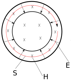
The consideration of the Poynting vector in static fields shows the relativistic nature of the Maxwell equations and allows a better understanding of the magnetic component of the Lorentz force, q(v × B). To illustrate, the accompanying picture is considered, which describes the Poynting vector in a cylindrical capacitor, which is located in an H field (pointing into the page) generated by a permanent magnet. Although there are only static electric and magnetic fields, the calculation of the Poynting vector produces a clockwise circular flow of electromagnetic energy, with no beginning or end.
While the circulating energy flow may seem unphysical, its existence is necessary to maintain conservation of angular momentum. The momentum of an electromagnetic wave in free space is equal to its power divided by c, the speed of light. Therefore, the circular flow of electromagnetic energy implies an angular momentum.[19] If one were to connect a wire between the two plates of the charged capacitor, then there would be a Lorentz force on that wire while the capacitor is discharging due to the discharge current and the crossed magnetic field; that force would be tangential to the central axis and thus add angular momentum to the system. That angular momentum would match the "hidden" angular momentum, revealed by the Poynting vector, circulating before the capacitor was discharged.
See also edit
References edit
- ^ Stratton, Julius Adams (1941). Electromagnetic Theory (1st ed.). New York: McGraw-Hill. ISBN 978-0-470-13153-4.
- ^ "Пойнтинга вектор". Физическая энциклопедия (in Russian). Retrieved 2022-02-21.
- ^ Nahin, Paul J. (2002). Oliver Heaviside: The Life, Work, and Times of an Electrical Genius of the Victorian Age. p. 131. ISBN 9780801869099.
- ^ Poynting, John Henry (1884). "On the Transfer of Energy in the Electromagnetic Field". Philosophical Transactions of the Royal Society of London. 175: 343–361. doi:10.1098/rstl.1884.0016.
- ^ Grant, Ian S.; Phillips, William R. (1990). Electromagnetism (2nd ed.). New York: John Wiley & Sons. ISBN 978-0-471-92712-9.
- ^ Griffiths, David J. (2012). Introduction to Electrodynamics (3rd ed.). Boston: Addison-Wesley. ISBN 978-0-321-85656-2.
- ^ Kinsler, Paul; Favaro, Alberto; McCall, Martin W. (2009). "Four Poynting Theorems". European Journal of Physics. 30 (5): 983. arXiv:0908.1721. Bibcode:2009EJPh...30..983K. doi:10.1088/0143-0807/30/5/007. S2CID 118508886.
- ^ Morton, N. (1979). "An Introduction to the Poynting Vector". Physics Education. 14 (5): 301–304. doi:10.1088/0031-9120/14/5/004.
- ^ a b Boulé, Marc (2024). "DC Power Transported by Two Infinite Parallel Wires". American Journal of Physics. 92 (1): 14–22. arXiv:2305.11827. doi:10.1119/5.0121399.
- ^ Pfeifer, Robert N. C.; Nieminen, Timo A.; Heckenberg, Norman R.; Rubinsztein-Dunlop, Halina (2007). "Momentum of an Electromagnetic Wave in Dielectric Media". Reviews of Modern Physics. 79 (4): 1197. arXiv:0710.0461. Bibcode:2007RvMP...79.1197P. doi:10.1103/RevModPhys.79.1197.
- ^ Umov, Nikolay Alekseevich (1874). "Ein Theorem über die Wechselwirkungen in Endlichen Entfernungen". Zeitschrift für Mathematik und Physik. 19: 97–114.
- ^ a b c d Jackson, John David (1998). Classical Electrodynamics (3rd ed.). New York: John Wiley & Sons. ISBN 978-0-471-30932-1.
- ^ "K. McDonald's Physics Examples - Railgun" (PDF). puhep1.princeton.edu. Retrieved 2021-02-14.
- ^ Zangwill, Andrew (2013). Modern Electrodynamics. Cambridge University Press. p. 508. ISBN 9780521896979.
- ^ a b Richter, Felix; Florian, Matthias; Henneberger, Klaus (2008). "Poynting's Theorem and Energy Conservation in the Propagation of Light in Bounded Media". EPL. 81 (6): 67005. arXiv:0710.0515. Bibcode:2008EL.....8167005R. doi:10.1209/0295-5075/81/67005. S2CID 119243693.
- ^ Harrington, Roger F. (2001). Time-Harmonic Electromagnetic Fields (2nd ed.). McGraw-Hill. ISBN 978-0-471-20806-8.
- ^ Hayt, William (2011). Engineering Electromagnetics (4th ed.). New York: McGraw-Hill. ISBN 978-0-07-338066-7.
- ^ Reitz, John R.; Milford, Frederick J.; Christy, Robert W. (2008). Foundations of Electromagnetic Theory (4th ed.). Boston: Addison-Wesley. ISBN 978-0-321-58174-7.
- ^ Feynman, Richard Phillips (2011). The Feynman Lectures on Physics. Vol. II: Mainly Electromagnetism and Matter (The New Millennium ed.). New York: Basic Books. ISBN 978-0-465-02494-0.
Further reading edit
- Becker, Richard (1982). Electromagnetic Fields and Interactions (1st ed.). Mineola, New York: Dover Publications. ISBN 978-0-486-64290-1.
- Edminister, Joseph; Nahvi, Mahmood (2013). Electromagnetics (4th ed.). New York: McGraw-Hill. ISBN 978-0-07-183149-9.