RLS was discovered by Gauss but lay unused or ignored until 1950 when Plackett rediscovered the original work of Gauss from 1821. In general, the RLS can be used to solve any problem that can be solved by adaptive filters. For example, suppose that a signal ${\displaystyle d(n)}$  is transmitted over an echoey, noisy channel that causes it to be received as

${\displaystyle x(n)=\sum _{k=0}^{q}b_{n}(k)d(n-k)+v(n)}$ 

where ${\displaystyle v(n)}$  represents additive noise. The intent of the RLS filter is to recover the desired signal ${\displaystyle d(n)}$  by use of a ${\displaystyle p+1}$ -tap FIR filter, ${\displaystyle \mathbf {w} }$ :

${\displaystyle d(n)\approx \sum _{k=0}^{p}w(k)x(n-k)=\mathbf {w} ^{\mathit {T}}\mathbf {x} _{n}}$ 

where ${\displaystyle \mathbf {x} _{n}=[x(n)\quad x(n-1)\quad \ldots \quad x(n-p)]^{T}}$  is the column vector containing the ${\displaystyle p+1}$  most recent samples of ${\displaystyle x(n)}$ . The estimate of the recovered desired signal is

${\displaystyle {\hat {d}}(n)=\sum _{k=0}^{p}w_{n}(k)x(n-k)=\mathbf {w} _{n}^{\mathit {T}}\mathbf {x} _{n}}$ 

The goal is to estimate the parameters of the filter ${\displaystyle \mathbf {w} }$ , and at each time ${\displaystyle n}$  we refer to the current estimate as ${\displaystyle \mathbf {w} _{n}}$  and the adapted least-squares estimate by ${\displaystyle \mathbf {w} _{n+1}}$ . ${\displaystyle \mathbf {w} _{n}}$  is also a column vector, as shown below, and the transpose, ${\displaystyle \mathbf {w} _{n}^{\mathit {T}}}$ , is a row vector. The matrix product ${\displaystyle \mathbf {w} _{n}^{\mathit {T}}\mathbf {x} _{n}}$  (which is the dot product of ${\displaystyle \mathbf {w} _{n}}$  and ${\displaystyle \mathbf {x} _{n}}$ ) is ${\displaystyle {\hat {d}}(n)}$ , a scalar. The estimate is "good" if ${\displaystyle {\hat {d}}(n)-d(n)}$  is small in magnitude in some least squares sense.

As time evolves, it is desired to avoid completely redoing the least squares algorithm to find the new estimate for ${\displaystyle \mathbf {w} _{n+1}}$ , in terms of ${\displaystyle \mathbf {w} _{n}}$ .

The benefit of the RLS algorithm is that there is no need to invert matrices, thereby saving computational cost. Another advantage is that it provides intuition behind such results as the Kalman filter.

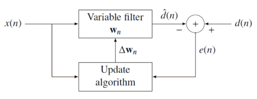
The idea behind RLS filters is to minimize a cost function ${\displaystyle C}$  by appropriately selecting the filter coefficients ${\displaystyle \mathbf {w} _{n}}$ , updating the filter as new data arrives. The error signal ${\displaystyle e(n)}$  and desired signal ${\displaystyle d(n)}$  are defined in the negative feedback diagram below:

The error implicitly depends on the filter coefficients through the estimate ${\displaystyle {\hat {d}}(n)}$ :

${\displaystyle e(n)=d(n)-{\hat {d}}(n)}$ 

The weighted least squares error function ${\displaystyle C}$ —the cost function we desire to minimize—being a function of ${\displaystyle e(n)}$  is therefore also dependent on the filter coefficients:

${\displaystyle C(\mathbf {w} _{n})=\sum _{i=0}^{n}\lambda ^{n-i}e^{2}(i)}$ 

where ${\displaystyle 0<\lambda \leq 1}$  is the "forgetting factor" which gives exponentially less weight to older error samples.

The cost function is minimized by taking the partial derivatives for all entries ${\displaystyle k}$  of the coefficient vector ${\displaystyle \mathbf {w} _{n}}$  and setting the results to zero

${\displaystyle {\frac {\partial C(\mathbf {w} _{n})}{\partial w_{n}(k)}}=\sum _{i=0}^{n}2\lambda ^{n-i}e(i)\cdot {\frac {\partial e(i)}{\partial w_{n}(k)}}=-\sum _{i=0}^{n}2\lambda ^{n-i}e(i)\,x(i-k)=0\qquad k=0,1,\ldots ,p}$ 

Next, replace ${\displaystyle e(n)}$  with the definition of the error signal

${\displaystyle \sum _{i=0}^{n}\lambda ^{n-i}\left[d(i)-\sum _{\ell =0}^{p}w_{n}(\ell )x(i-\ell )\right]x(i-k)=0\qquad k=0,1,\ldots ,p}$ 

Rearranging the equation yields

${\displaystyle \sum _{\ell =0}^{p}w_{n}(\ell )\left[\sum _{i=0}^{n}\lambda ^{n-i}\,x(i-l)x(i-k)\right]=\sum _{i=0}^{n}\lambda ^{n-i}d(i)x(i-k)\qquad k=0,1,\ldots ,p}$ 

This form can be expressed in terms of matrices

${\displaystyle \mathbf {R} _{x}(n)\,\mathbf {w} _{n}=\mathbf {r} _{dx}(n)}$ 

where ${\displaystyle \mathbf {R} _{x}(n)}$  is the weighted sample covariance matrix for ${\displaystyle x(n)}$ , and ${\displaystyle \mathbf {r} _{dx}(n)}$  is the equivalent estimate for the cross-covariance between ${\displaystyle d(n)}$  and ${\displaystyle x(n)}$ . Based on this expression we find the coefficients which minimize the cost function as

${\displaystyle \mathbf {w} _{n}=\mathbf {R} _{x}^{-1}(n)\,\mathbf {r} _{dx}(n)}$ 

This is the main result of the discussion.

Choosing λ edit

The smaller ${\displaystyle \lambda }$  is, the smaller is the contribution of previous samples to the covariance matrix. This makes the filter more sensitive to recent samples, which means more fluctuations in the filter co-efficients. The ${\displaystyle \lambda =1}$  case is referred to as the growing window RLS algorithm. In practice, ${\displaystyle \lambda }$  is usually chosen between 0.98 and 1.^[1] By using type-II maximum likelihood estimation the optimal ${\displaystyle \lambda }$  can be estimated from a set of data.^[2]

The discussion resulted in a single equation to determine a coefficient vector which minimizes the cost function. In this section we want to derive a recursive solution of the form

${\displaystyle \mathbf {w} _{n}=\mathbf {w} _{n-1}+\Delta \mathbf {w} _{n-1}}$ 

where ${\displaystyle \Delta \mathbf {w} _{n-1}}$  is a correction factor at time ${\displaystyle {n-1}}$ . We start the derivation of the recursive algorithm by expressing the cross covariance ${\displaystyle \mathbf {r} _{dx}(n)}$  in terms of ${\displaystyle \mathbf {r} _{dx}(n-1)}$ 

${\displaystyle \mathbf {r} _{dx}(n)}$	${\displaystyle =\sum _{i=0}^{n}\lambda ^{n-i}d(i)\mathbf {x} (i)}$
	${\displaystyle =\sum _{i=0}^{n-1}\lambda ^{n-i}d(i)\mathbf {x} (i)+\lambda ^{0}d(n)\mathbf {x} (n)}$
	${\displaystyle =\lambda \mathbf {r} _{dx}(n-1)+d(n)\mathbf {x} (n)}$

where ${\displaystyle \mathbf {x} (i)}$  is the ${\displaystyle {p+1}}$  dimensional data vector

${\displaystyle \mathbf {x} (i)=[x(i),x(i-1),\dots ,x(i-p)]^{T}}$ 

Similarly we express ${\displaystyle \mathbf {R} _{x}(n)}$  in terms of ${\displaystyle \mathbf {R} _{x}(n-1)}$  by

${\displaystyle \mathbf {R} _{x}(n)}$	${\displaystyle =\sum _{i=0}^{n}\lambda ^{n-i}\mathbf {x} (i)\mathbf {x} ^{T}(i)}$
	${\displaystyle =\lambda \mathbf {R} _{x}(n-1)+\mathbf {x} (n)\mathbf {x} ^{T}(n)}$

In order to generate the coefficient vector we are interested in the inverse of the deterministic auto-covariance matrix. For that task the Woodbury matrix identity comes in handy. With

${\displaystyle A}$	${\displaystyle =\lambda \mathbf {R} _{x}(n-1)}$  is ${\displaystyle (p+1)}$ -by-${\displaystyle (p+1)}$
${\displaystyle U}$	${\displaystyle =\mathbf {x} (n)}$  is ${\displaystyle (p+1)}$ -by-1 (column vector)
${\displaystyle V}$	${\displaystyle =\mathbf {x} ^{T}(n)}$  is 1-by-${\displaystyle (p+1)}$  (row vector)
${\displaystyle C}$	${\displaystyle =\mathbf {I} _{1}}$  is the 1-by-1 identity matrix

The Woodbury matrix identity follows

${\displaystyle \mathbf {R} _{x}^{-1}(n)}$	${\displaystyle =}$	${\displaystyle \left[\lambda \mathbf {R} _{x}(n-1)+\mathbf {x} (n)\mathbf {x} ^{T}(n)\right]^{-1}}$
	${\displaystyle =}$	${\displaystyle {\dfrac {1}{\lambda }}\left\lbrace \mathbf {R} _{x}^{-1}(n-1)-{\dfrac {\mathbf {R} _{x}^{-1}(n-1)\mathbf {x} (n)\mathbf {x} ^{T}(n)\mathbf {R} _{x}^{-1}(n-1)}{\lambda +\mathbf {x} ^{T}(n)\mathbf {R} _{x}^{-1}(n-1)\mathbf {x} (n)}}\right\rbrace }$
		${\displaystyle }$

To come in line with the standard literature, we define

${\displaystyle \mathbf {P} (n)}$	${\displaystyle =\mathbf {R} _{x}^{-1}(n)}$
	${\displaystyle =\lambda ^{-1}\mathbf {P} (n-1)-\mathbf {g} (n)\mathbf {x} ^{T}(n)\lambda ^{-1}\mathbf {P} (n-1)}$

where the gain vector ${\displaystyle g(n)}$  is

${\displaystyle \mathbf {g} (n)}$	${\displaystyle =\lambda ^{-1}\mathbf {P} (n-1)\mathbf {x} (n)\left\{1+\mathbf {x} ^{T}(n)\lambda ^{-1}\mathbf {P} (n-1)\mathbf {x} (n)\right\}^{-1}}$
	${\displaystyle =\mathbf {P} (n-1)\mathbf {x} (n)\left\{\lambda +\mathbf {x} ^{T}(n)\mathbf {P} (n-1)\mathbf {x} (n)\right\}^{-1}}$

Before we move on, it is necessary to bring ${\displaystyle \mathbf {g} (n)}$  into another form

${\displaystyle \mathbf {g} (n)\left\{1+\mathbf {x} ^{T}(n)\lambda ^{-1}\mathbf {P} (n-1)\mathbf {x} (n)\right\}}$	${\displaystyle =\lambda ^{-1}\mathbf {P} (n-1)\mathbf {x} (n)}$
${\displaystyle \mathbf {g} (n)+\mathbf {g} (n)\mathbf {x} ^{T}(n)\lambda ^{-1}\mathbf {P} (n-1)\mathbf {x} (n)}$	${\displaystyle =\lambda ^{-1}\mathbf {P} (n-1)\mathbf {x} (n)}$

Subtracting the second term on the left side yields

${\displaystyle \mathbf {g} (n)}$	${\displaystyle =\lambda ^{-1}\mathbf {P} (n-1)\mathbf {x} (n)-\mathbf {g} (n)\mathbf {x} ^{T}(n)\lambda ^{-1}\mathbf {P} (n-1)\mathbf {x} (n)}$
	${\displaystyle =\lambda ^{-1}\left[\mathbf {P} (n-1)-\mathbf {g} (n)\mathbf {x} ^{T}(n)\mathbf {P} (n-1)\right]\mathbf {x} (n)}$

With the recursive definition of ${\displaystyle \mathbf {P} (n)}$  the desired form follows

${\displaystyle \mathbf {g} (n)=\mathbf {P} (n)\mathbf {x} (n)}$ 

Now we are ready to complete the recursion. As discussed

${\displaystyle \mathbf {w} _{n}}$	${\displaystyle =\mathbf {P} (n)\,\mathbf {r} _{dx}(n)}$
	${\displaystyle =\lambda \mathbf {P} (n)\,\mathbf {r} _{dx}(n-1)+d(n)\mathbf {P} (n)\,\mathbf {x} (n)}$

The second step follows from the recursive definition of ${\displaystyle \mathbf {r} _{dx}(n)}$ . Next we incorporate the recursive definition of ${\displaystyle \mathbf {P} (n)}$  together with the alternate form of ${\displaystyle \mathbf {g} (n)}$  and get

${\displaystyle \mathbf {w} _{n}}$	${\displaystyle =\lambda \left[\lambda ^{-1}\mathbf {P} (n-1)-\mathbf {g} (n)\mathbf {x} ^{T}(n)\lambda ^{-1}\mathbf {P} (n-1)\right]\mathbf {r} _{dx}(n-1)+d(n)\mathbf {g} (n)}$
	${\displaystyle =\mathbf {P} (n-1)\mathbf {r} _{dx}(n-1)-\mathbf {g} (n)\mathbf {x} ^{T}(n)\mathbf {P} (n-1)\mathbf {r} _{dx}(n-1)+d(n)\mathbf {g} (n)}$
	${\displaystyle =\mathbf {P} (n-1)\mathbf {r} _{dx}(n-1)+\mathbf {g} (n)\left[d(n)-\mathbf {x} ^{T}(n)\mathbf {P} (n-1)\mathbf {r} _{dx}(n-1)\right]}$

With ${\displaystyle \mathbf {w} _{n-1}=\mathbf {P} (n-1)\mathbf {r} _{dx}(n-1)}$  we arrive at the update equation

${\displaystyle \mathbf {w} _{n}}$	${\displaystyle =\mathbf {w} _{n-1}+\mathbf {g} (n)\left[d(n)-\mathbf {x} ^{T}(n)\mathbf {w} _{n-1}\right]}$
	${\displaystyle =\mathbf {w} _{n-1}+\mathbf {g} (n)\alpha (n)}$

where ${\displaystyle \alpha (n)=d(n)-\mathbf {x} ^{T}(n)\mathbf {w} _{n-1}}$  is the a priori error. Compare this with the a posteriori error; the error calculated after the filter is updated:

${\displaystyle e(n)=d(n)-\mathbf {x} ^{T}(n)\mathbf {w} _{n}}$ 

That means we found the correction factor

${\displaystyle \Delta \mathbf {w} _{n-1}=\mathbf {g} (n)\alpha (n)}$ 

This intuitively satisfying result indicates that the correction factor is directly proportional to both the error and the gain vector, which controls how much sensitivity is desired, through the weighting factor, ${\displaystyle \lambda }$ .

The RLS algorithm for a p-th order RLS filter can be summarized as

The recursion for ${\displaystyle P}$  follows an algebraic Riccati equation and thus draws parallels to the Kalman filter.^[3]

The lattice recursive least squares adaptive filter is related to the standard RLS except that it requires fewer arithmetic operations (order N).^[4] It offers additional advantages over conventional LMS algorithms such as faster convergence rates, modular structure, and insensitivity to variations in eigenvalue spread of the input correlation matrix. The LRLS algorithm described is based on a posteriori errors and includes the normalized form. The derivation is similar to the standard RLS algorithm and is based on the definition of ${\displaystyle d(k)\,\!}$ . In the forward prediction case, we have ${\displaystyle d(k)=x(k)\,\!}$  with the input signal ${\displaystyle x(k-1)\,\!}$  as the most up to date sample. The backward prediction case is ${\displaystyle d(k)=x(k-i-1)\,\!}$ , where i is the index of the sample in the past we want to predict, and the input signal ${\displaystyle x(k)\,\!}$  is the most recent sample.^[5]

Parameter summary edit

${\displaystyle \kappa _{f}(k,i)\,\!}$  is the forward reflection coefficient

${\displaystyle \kappa _{b}(k,i)\,\!}$  is the backward reflection coefficient

${\displaystyle e_{f}(k,i)\,\!}$  represents the instantaneous a posteriori forward prediction error

${\displaystyle e_{b}(k,i)\,\!}$  represents the instantaneous a posteriori backward prediction error

${\displaystyle \xi _{b_{\min }}^{d}(k,i)\,\!}$  is the minimum least-squares backward prediction error

${\displaystyle \xi _{f_{\min }}^{d}(k,i)\,\!}$  is the minimum least-squares forward prediction error

${\displaystyle \gamma (k,i)\,\!}$  is a conversion factor between a priori and a posteriori errors

${\displaystyle v_{i}(k)\,\!}$  are the feedforward multiplier coefficients.

${\displaystyle \varepsilon \,\!}$  is a small positive constant that can be 0.01

LRLS algorithm summary edit

The algorithm for a LRLS filter can be summarized as

The normalized form of the LRLS has fewer recursions and variables. It can be calculated by applying a normalization to the internal variables of the algorithm which will keep their magnitude bounded by one. This is generally not used in real-time applications because of the number of division and square-root operations which comes with a high computational load.

NLRLS algorithm summary edit

The algorithm for a NLRLS filter can be summarized as

• Adaptive filter
• Kernel adaptive filter
• Least mean squares filter
• Zero-forcing equalizer

• Hayes, Monson H. (1996). "9.4: Recursive Least Squares". Statistical Digital Signal Processing and Modeling. Wiley. p. 541. ISBN 0-471-59431-8.
• Simon Haykin, Adaptive Filter Theory, Prentice Hall, 2002, ISBN 0-13-048434-2
• M.H.A Davis, R.B. Vinter, Stochastic Modelling and Control, Springer, 1985, ISBN 0-412-16200-8
• Weifeng Liu, Jose Principe and Simon Haykin, Kernel Adaptive Filtering: A Comprehensive Introduction, John Wiley, 2010, ISBN 0-470-44753-2
• R.L.Plackett, Some Theorems in Least Squares, Biometrika, 1950, 37, 149–157, ISSN 0006-3444
• C.F.Gauss, Theoria combinationis observationum erroribus minimis obnoxiae, 1821, Werke, 4. Gottinge