Shooting_method Knowpia

In numerical analysis, the shooting method is a method for solving a boundary value problem by reducing it to an initial value problem. It involves finding solutions to the initial value problem for different initial conditions until one finds the solution that also satisfies the boundary conditions of the boundary value problem. In layman's terms, one "shoots" out trajectories in different directions from one boundary until one finds the trajectory that "hits" the other boundary condition.

Mathematical description edit

Suppose one wants to solve the boundary-value problem

y''(t)=f(t,y(t),y'(t)),\quad y(t_{0})=y_{0},\quad y(t_{1})=y_{1}.

Let

y(t;a)

solve the initial-value problem

y''(t)=f(t,y(t),y'(t)),\quad y(t_{0})=y_{0},\quad y'(t_{0})=a.

If

y(t_{1};a)=y_{1}

, then

y(t;a)

is also a solution of the boundary-value problem.

The shooting method is the process of solving the initial value problem for many different values of $a$ until one finds the solution $y(t;a)$ that satisfies the desired boundary conditions. Typically, one does so numerically. The solution(s) correspond to root(s) of

F(a)=y(t_{1};a)-y_{1}.

To systematically vary the shooting parameter

a

and find the root, one can employ standard root-finding algorithms like the bisection method or Newton's method.

Roots of $F$ and solutions to the boundary value problem are equivalent. If $a$ is a root of $F$ , then $y(t;a)$ is a solution of the boundary value problem. Conversely, if the boundary value problem has a solution $y(t)$ , it is also the unique solution $y(t;a)$ of the initial value problem where $a=y'(t_{0})$ , so $a$ is a root of $F$ .

Etymology and intuition edit

The term "shooting method" has its origin in artillery. An analogy for the shooting method is to

place a cannon at the position $y(t_{0})=y_{0}$ , then
vary the angle $a=y'(t_{0})$ of the cannon, then
fire the cannon until it hits the boundary value $y(t_{1})=y_{1}$ .

Between each shot, the direction of the cannon is adjusted based on the previous shot, so every shot hits closer than the previous one. The trajectory that "hits" the desired boundary value is the solution to the boundary value problem — hence the name "shooting method".

Linear shooting method edit

The boundary value problem is linear if f has the form

f(t,y(t),y'(t))=p(t)y'(t)+q(t)y(t)+r(t).

In this case, the solution to the boundary value problem is usually given by:

y(t)=y_{(1)}(t)+{\frac {y_{1}-y_{(1)}(t_{1})}{y_{(2)}(t_{1})}}y_{(2)}(t)

where

y_{(1)}(t)

is the solution to the initial value problem:

y_{(1)}''(t)=p(t)y_{(1)}'(t)+q(t)y_{(1)}(t)+r(t),\quad y_{(1)}(t_{0})=y_{0},\quad y_{(1)}'(t_{0})=0,

and

y_{(2)}(t)

is the solution to the initial value problem:

y_{(2)}''(t)=p(t)y_{(2)}'(t)+q(t)y_{(2)}(t),\quad y_{(2)}(t_{0})=0,\quad y_{(2)}'(t_{0})=1.

See the proof for the precise condition under which this result holds.^[1]

Examples edit

Standard boundary value problem edit

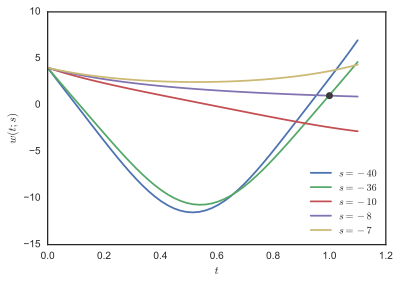
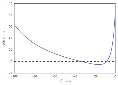
Figure 1. Trajectories w(t;s) for s = w'(0) equal to −7, −8, −10, −36, and −40. The point (1,1) is marked with a circle.

Figure 2. The function F(s) = w(1;s) − 1.

A boundary value problem is given as follows by Stoer and Bulirsch^[2] (Section 7.3.1).

w''(t)={\frac {3}{2}}w^{2}(t),\quad w(0)=4,\quad w(1)=1

The initial value problem

w''(t)={\frac {3}{2}}w^{2}(t),\quad w(0)=4,\quad w'(0)=s

was solved for s = −1, −2, −3, ..., −100, and F(s) = w(1;s) − 1 plotted in the Figure 2. Inspecting the plot of F, we see that there are roots near −8 and −36. Some trajectories of w(t;s) are shown in the Figure 1.

Stoer and Bulirsch^[2] state that there are two solutions, which can be found by algebraic methods.

These correspond to the initial conditions w′(0) = −8 and w′(0) = −35.9 (approximately).

Eigenvalue problem edit

When searching for the ground state of the harmonic oscillator with energy

E_{0}=1/2

, the shooting method produces wavefunctions that diverge to infinity. Here, the correct wavefunction should have zero roots and go to zero at infinity, so it lies somewhere between the orange and green lines. The energy is therefore between

0.495

and

0.500

(with numerical accuracy).

The shooting method can also be used to solve eigenvalue problems. Consider the time-independent Schrödinger equation for the quantum harmonic oscillator

-{\frac {1}{2}}\psi _{n}''(x)+{\frac {1}{2}}x^{2}\psi _{n}(x)=E_{n}\psi _{n}(x).

In quantum mechanics, one seeks normalizable wavefunctions

\psi _{n}(x)

and their corresponding energies subject to the boundary conditions

\psi _{n}(x\rightarrow +\infty )=\psi _{n}(x\rightarrow -\infty )=0.

The problem can be solved analytically to find the energies

E_{n}=n+1/2

for

n=0,1,2,\dots

, but also serves as an excellent illustration of the shooting method. To apply it, first note some general properties of the Schrödinger equation:

If $\psi _{n}(x)$ is an eigenfunction, so is $C\psi _{n}(x)$ for any nonzero constant $C$ .
The $n$ -th excited state $\psi _{n}(x)$ has $n$ roots where $\psi _{n}(x)=0$ .
For even $n$ , the $n$ -th excited state $\psi _{n}(x)=\psi _{n}(-x)$ is symmetric and nonzero at the origin.
For odd $n$ , the $n$ -th excited state $\psi _{n}(x)=-\psi _{n}(-x)$ is antisymmetric and thus zero at the origin.

To find the $n$ -th excited state $\psi _{n}(x)$ and its energy $E_{n}$ , the shooting method is then to:

Guess some energy $E_{n}$ .
Integrate the Schrödinger equation. For example, use the central finite difference
$-{\frac {1}{2}}{\frac {\psi _{n}^{i+1}-2\psi _{n}^{i}+\psi _{n}^{i-1}}{{\Delta x}^{2}}}+{\frac {1}{2}}(x^{i})^{2}\psi _{n}^{i}=E_{n}\psi _{n}^{i}.$
- If $n$ is even, set $\psi _{0}$ to some arbitrary number (say $\psi _{n}^{0}=1$ — the wavefunction can be normalized after integration anyway) and use the symmetric property to find all remaining $\psi _{n}^{i}$ .
- If $n$ is odd, set $\psi _{n}^{0}=0$ and $\psi _{n}^{1}$ to some arbitrary number (say $\psi _{n}^{1}=1$ — the wavefunction can be normalized after integration anyway) and find all remaining $\psi _{n}^{i}$ .
Count the roots of $\psi _{n}$ and refine the guess for the energy $E_{n}$ .
- If there are $n$ or less roots, the guessed energy is too low, so increase it and repeat the process.
- If there are more than $n$ roots, the guessed energy is too high, so decrease it and repeat the process.

The energy-guessing can be done with the bisection method, and the process can be terminated when the energy difference is sufficiently small. Then one can take any energy in the interval to be the correct energy.

Notes edit

^ Mathews, John H.; Fink, Kurtis K. (2004). "9.8 Boundary Value Problems". Numerical methods using MATLAB (PDF) (4th ed.). Upper Saddle River, N.J.: Pearson. ISBN 0-13-065248-2. Archived from the original (PDF) on 9 December 2006.
^ ^a ^b Stoer, J. and Bulirsch, R. Introduction to Numerical Analysis. New York: Springer-Verlag, 1980.

References edit

Press, WH; Teukolsky, SA; Vetterling, WT; Flannery, BP (2007). "Section 18.1. The Shooting Method". Numerical Recipes: The Art of Scientific Computing (3rd ed.). New York: Cambridge University Press. ISBN 978-0-521-88068-8.

External links edit

Brief Description of ODEPACK (at Netlib; contains LSODE)
Shooting method of solving boundary value problems – Notes, PPT, Maple, Mathcad, Matlab, Mathematica at Holistic Numerical Methods Institute [1]