


Summary
In electrical engineering, a transmission line is a specialized cable or other structure designed to conduct electromagnetic waves in a contained manner. The term applies when the conductors are long enough that the wave nature of the transmission must be taken into account. This applies especially to radio-frequency engineering because the short wavelengths mean that wave phenomena arise over very short distances (this can be as short as millimetres depending on frequency). However, the theory of transmission lines was historically developed to explain phenomena on very long telegraph lines, especially submarine telegraph cables.
Transmission lines are used for purposes such as connecting radio transmitters and receivers with their antennas (they are then called feed lines or feeders), distributing cable television signals, trunklines routing calls between telephone switching centres, computer network connections and high speed computer data buses. RF engineers commonly use short pieces of transmission line, usually in the form of printed planar transmission lines, arranged in certain patterns to build circuits such as filters. These circuits, known as distributed-element circuits, are an alternative to traditional circuits using discrete capacitors and inductors.
Overview edit
Ordinary electrical cables suffice to carry low frequency alternating current (AC), such as mains power, which reverses direction 100 to 120 times per second, and audio signals. However, they not generally used to carry currents in the radio frequency range,[1] above about 30 kHz, because the energy tends to radiate off the cable as radio waves, causing power losses. Radio frequency currents also tend to reflect from discontinuities in the cable such as connectors and joints, and travel back down the cable toward the source.[1][2] These reflections act as bottlenecks, preventing the signal power from reaching the destination. Transmission lines use specialized construction, and impedance matching, to carry electromagnetic signals with minimal reflections and power losses. The distinguishing feature of most transmission lines is that they have uniform cross sectional dimensions along their length, giving them a uniform impedance, called the characteristic impedance,[2][3][4] to prevent reflections. Types of transmission line include parallel line (ladder line, twisted pair), coaxial cable, and planar transmission lines such as stripline and microstrip.[5][6] The higher the frequency of electromagnetic waves moving through a given cable or medium, the shorter the wavelength of the waves. Transmission lines become necessary when the transmitted frequency's wavelength is sufficiently short that the length of the cable becomes a significant part of a wavelength.
At microwave frequencies and above, power losses in transmission lines become excessive, and waveguides are used instead,[1] which function as "pipes" to confine and guide the electromagnetic waves.[6] Some sources define waveguides as a type of transmission line;[6] however, this article will not include them.
History edit
Mathematical analysis of the behaviour of electrical transmission lines grew out of the work of James Clerk Maxwell, Lord Kelvin, and Oliver Heaviside. In 1855, Lord Kelvin formulated a diffusion model of the current in a submarine cable. The model correctly predicted the poor performance of the 1858 trans-Atlantic submarine telegraph cable. In 1885, Heaviside published the first papers that described his analysis of propagation in cables and the modern form of the telegrapher's equations.[7]
The four terminal model edit
For the purposes of analysis, an electrical transmission line can be modelled as a two-port network (also called a quadripole), as follows:
![]()
In the simplest case, the network is assumed to be linear (i.e. the complex voltage across either port is proportional to the complex current flowing into it when there are no reflections), and the two ports are assumed to be interchangeable. If the transmission line is uniform along its length, then its behaviour is largely described by a two parameters called characteristic impedance, symbol Z0 and propagation delay, symbol . Z0 is the ratio of the complex voltage of a given wave to the complex current of the same wave at any point on the line. Typical values of Z0 are 50 or 75 ohms for a coaxial cable, about 100 ohms for a twisted pair of wires, and about 300 ohms for a common type of untwisted pair used in radio transmission. Propagation delay is proportional to the length of the transmission line and is never less than the length divided by the speed of light. Typical delays for modern communication transmission lines vary from 3.33 ns/m to 5 ns/m.

When sending power down a transmission line, it is usually desirable that as much power as possible will be absorbed by the load and as little as possible will be reflected back to the source. This can be ensured by making the load impedance equal to Z0, in which case the transmission line is said to be matched.
Some of the power that is fed into a transmission line is lost because of its resistance. This effect is called ohmic or resistive loss (see ohmic heating). At high frequencies, another effect called dielectric loss becomes significant, adding to the losses caused by resistance. Dielectric loss is caused when the insulating material inside the transmission line absorbs energy from the alternating electric field and converts it to heat (see dielectric heating). The transmission line is modelled with a resistance (R) and inductance (L) in series with a capacitance (C) and conductance (G) in parallel. The resistance and conductance contribute to the loss in a transmission line.
The total loss of power in a transmission line is often specified in decibels per metre (dB/m), and usually depends on the frequency of the signal. The manufacturer often supplies a chart showing the loss in dB/m at a range of frequencies. A loss of 3 dB corresponds approximately to a halving of the power.
Propagation delay is often specified in units of nanoseconds per metre. While propagation delay usually depends on the frequency of the signal, transmission lines are typically operated over frequency ranges where the propagation delay is approximately constant.
Telegrapher's equations edit
The telegrapher's equations (or just telegraph equations) are a pair of linear differential equations which describe the voltage ( ) and current ( ) on an electrical transmission line with distance and time. They were developed by Oliver Heaviside who created the transmission line model, and are based on Maxwell's equations.


The transmission line model is an example of the distributed-element model. It represents the transmission line as an infinite series of two-port elementary components, each representing an infinitesimally short segment of the transmission line:
- The distributed resistance of the conductors is represented by a series resistor (expressed in ohms per unit length).
- The distributed inductance (due to the magnetic field around the wires, self-inductance, etc.) is represented by a series inductor (in henries per unit length).
- The capacitance between the two conductors is represented by a shunt capacitor (in farads per unit length).
- The conductance of the dielectric material separating the two conductors is represented by a shunt resistor between the signal wire and the return wire (in siemens per unit length).


The model consists of an infinite series of the elements shown in the figure, and the values of the components are specified per unit length so the picture of the component can be misleading. , , , and may also be functions of frequency. An alternative notation is to use , , and to emphasize that the values are derivatives with respect to length. These quantities can also be known as the primary line constants to distinguish from the secondary line constants derived from them, these being the propagation constant, attenuation constant and phase constant.


The line voltage and the current can be expressed in the frequency domain as


- (see differential equation, angular frequency ω and imaginary unit j)
Special case of a lossless line edit
When the elements and are negligibly small the transmission line is considered as a lossless structure. In this hypothetical case, the model depends only on the and elements which greatly simplifies the analysis. For a lossless transmission line, the second order steady-state Telegrapher's equations are:


These are wave equations which have plane waves with equal propagation speed in the forward and reverse directions as solutions. The physical significance of this is that electromagnetic waves propagate down transmission lines and in general, there is a reflected component that interferes with the original signal. These equations are fundamental to transmission line theory.
General case of a line with losses edit
In the general case the loss terms, and , are both included, and the full form of the Telegrapher's equations become:


where is the (complex) propagation constant. These equations are fundamental to transmission line theory. They are also wave equations, and have solutions similar to the special case, but which are a mixture of sines and cosines with exponential decay factors. Solving for the propagation constant in terms of the primary parameters , , , and gives:


and the characteristic impedance can be expressed as

The solutions for and are:


The constants must be determined from boundary conditions. For a voltage pulse , starting at and moving in the positive direction, then the transmitted pulse at position can be obtained by computing the Fourier Transform, , of , attenuating each frequency component by , advancing its phase by , and taking the inverse Fourier Transform. The real and imaginary parts of can be computed as


with
![{\displaystyle a~\equiv ~R\,G\,-\omega ^{2}L\,C\ ~=~\omega ^{2}L\,C\,\left[\left({\frac {R}{\omega L}}\right)\left({\frac {G}{\omega C}}\right)-1\right]}](https://wikimedia.org/api/rest_v1/media/math/render/svg/4cef639bb12081b0b0eac890fc86424b1a1030e9)

the right-hand expressions holding when neither , nor , nor is zero, and with


where atan2 is the everywhere-defined form of two-parameter arctangent function, with arbitrary value zero when both arguments are zero.
Alternatively, the complex square root can be evaluated algebraically, to yield:

and

with the plus or minus signs chosen opposite to the direction of the wave's motion through the conducting medium. (a is usually negative, since and are typically much smaller than and , respectively, so −a is usually positive. b is always positive.)


Special, low loss case edit
For small losses and high frequencies, the general equations can be simplified: If and then


Since an advance in phase by is equivalent to a time delay by , can be simply computed as


Heaviside condition edit
The Heaviside condition is .

If R, G, L, and C are constants that are not frequency dependent and the Heaviside condition is met, then waves travel down the transmission line without dispersion distortion.
Input impedance of transmission line edit


The characteristic impedance of a transmission line is the ratio of the amplitude of a single voltage wave to its current wave. Since most transmission lines also have a reflected wave, the characteristic impedance is generally not the impedance that is measured on the line.

The impedance measured at a given distance from the load impedance may be expressed as

- ,

where is the propagation constant and is the voltage reflection coefficient measured at the load end of the transmission line. Alternatively, the above formula can be rearranged to express the input impedance in terms of the load impedance rather than the load voltage reflection coefficient:

- .

Input impedance of lossless transmission line edit
For a lossless transmission line, the propagation constant is purely imaginary, , so the above formulas can be rewritten as


where is the wavenumber.

In calculating the wavelength is generally different inside the transmission line to what it would be in free-space. Consequently, the velocity factor of the material the transmission line is made of needs to be taken into account when doing such a calculation.

Special cases of lossless transmission lines edit
Half wave length edit
For the special case where where n is an integer (meaning that the length of the line is a multiple of half a wavelength), the expression reduces to the load impedance so that


for all This includes the case when , meaning that the length of the transmission line is negligibly small compared to the wavelength. The physical significance of this is that the transmission line can be ignored (i.e. treated as a wire) in either case.


Quarter wave length edit
For the case where the length of the line is one quarter wavelength long, or an odd multiple of a quarter wavelength long, the input impedance becomes

Matched load edit
Another special case is when the load impedance is equal to the characteristic impedance of the line (i.e. the line is matched), in which case the impedance reduces to the characteristic impedance of the line so that

for all and all .

Short edit
For the case of a shorted load (i.e. ), the input impedance is purely imaginary and a periodic function of position and wavelength (frequency)


Open edit
For the case of an open load (i.e. ), the input impedance is once again imaginary and periodic


Matrix parameters edit
The simulation of transmission lines embedded into larger systems generally utilize admittance parameters (Y matrix), impedance parameters (Z matrix), and/or scattering parameters (S matrix) that embodies the full transmission line model needed to support the simulation.
Admittance parameters edit
Admittance (Y) parameters may be defined by applying a fixed voltage to one port (V1) of a transmission line with the other end shorted to ground and measuring the resulting current running into each port (I1, I2)[8][9] and computing the admittance on each port as a ratio of I/V The admittance parameter Y11 is I1/V1, and the admittance parameter Y12 is I2/V1. Since transmission lines are electrically passive and symmetric devices, Y12 = Y21, and Y11 = Y22.
For lossless and lossy transmission lines respectively, the Y parameter matrix is as follows:[10][11]

Impedance parameters edit
Impedance (Z) parameter may defines by applying a fixed current into one port (I1) of a transmission line with the other port open and measuring the resulting voltage on each port (V1, V2)[8][9] and computing the impedance parameter Z11 is V1/I1, and the impedance parameter Z12 is V2/I1. Since transmission lines are electrically passive and symmetric devices, V12 = V21, and V11 = V22.
In the Y and Z matrix definitions, and .[12] Unlike ideal lumped 2 port elements (resistors, capacitors, inductors, etc.) which do not have defined Z parameters, transmission lines have an internal path to ground, which permits the definition of Z parameters.


For lossless and lossy transmission lines respectively, the Z parameter matrix is as follows:[10][11]

Scattering parameters edit
Scattering (S) matrix parameters model the electrical behavior of the transmission line with matched loads at each termination.[10]
For lossless and lossy transmission lines respectively, the S parameter matrix is as follows,[13][14] using standard hyperbolic to circular complex translations.

Variable definitions edit
In all matrix parameters above, the following variable definitions apply:

Zp = port impedance, or termination impedance
= the propagation constant per unit length

= attenuation constant in nepers per unit length

= wave number or phase constant radians per unit length

= frequency radians / second

= wave length in unit length
L = inductance per unit length
C = capacitance per unit length
= effective dielectric constant

= 299,792,458 meters / second = Speed of light in a vacuum

Practical types edit
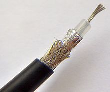
Coaxial cable edit
Coaxial lines confine virtually all of the electromagnetic wave to the area inside the cable. Coaxial lines can therefore be bent and twisted (subject to limits) without negative effects, and they can be strapped to conductive supports without inducing unwanted currents in them. In radio-frequency applications up to a few gigahertz, the wave propagates in the transverse electric and magnetic mode (TEM) only, which means that the electric and magnetic fields are both perpendicular to the direction of propagation (the electric field is radial, and the magnetic field is circumferential). However, at frequencies for which the wavelength (in the dielectric) is significantly shorter than the circumference of the cable other transverse modes can propagate. These modes are classified into two groups, transverse electric (TE) and transverse magnetic (TM) waveguide modes. When more than one mode can exist, bends and other irregularities in the cable geometry can cause power to be transferred from one mode to another.
The most common use for coaxial cables is for television and other signals with bandwidth of multiple megahertz. In the middle 20th century they carried long distance telephone connections.
Planar lines edit
Planar transmission lines are transmission lines with conductors, or in some cases dielectric strips, that are flat, ribbon-shaped lines. They are used to interconnect components on printed circuits and integrated circuits working at microwave frequencies because the planar type fits in well with the manufacturing methods for these components. Several forms of planar transmission lines exist.
Microstrip edit
A microstrip circuit uses a thin flat conductor which is parallel to a ground plane. Microstrip can be made by having a strip of copper on one side of a printed circuit board (PCB) or ceramic substrate while the other side is a continuous ground plane. The width of the strip, the thickness of the insulating layer (PCB or ceramic) and the dielectric constant of the insulating layer determine the characteristic impedance. Microstrip is an open structure whereas coaxial cable is a closed structure.
Stripline edit
A stripline circuit uses a flat strip of metal which is sandwiched between two parallel ground planes. The insulating material of the substrate forms a dielectric. The width of the strip, the thickness of the substrate and the relative permittivity of the substrate determine the characteristic impedance of the strip which is a transmission line.
Coplanar waveguide edit
A coplanar waveguide consists of a center strip and two adjacent outer conductors, all three of them flat structures that are deposited onto the same insulating substrate and thus are located in the same plane ("coplanar"). The width of the center conductor, the distance between inner and outer conductors, and the relative permittivity of the substrate determine the characteristic impedance of the coplanar transmission line.
Balanced lines edit
A balanced line is a transmission line consisting of two conductors of the same type, and equal impedance to ground and other circuits. There are many formats of balanced lines, amongst the most common are twisted pair, star quad and twin-lead.
Twisted pair edit
Twisted pairs are commonly used for terrestrial telephone communications. In such cables, many pairs are grouped together in a single cable, from two to several thousand.[15] The format is also used for data network distribution inside buildings, but the cable is more expensive because the transmission line parameters are tightly controlled.
Star quad edit
Star quad is a four-conductor cable in which all four conductors are twisted together around the cable axis. It is sometimes used for two circuits, such as 4-wire telephony and other telecommunications applications. In this configuration each pair uses two non-adjacent conductors. Other times it is used for a single, balanced line, such as audio applications and 2-wire telephony. In this configuration two non-adjacent conductors are terminated together at both ends of the cable, and the other two conductors are also terminated together.
When used for two circuits, crosstalk is reduced relative to cables with two separate twisted pairs.
When used for a single, balanced line, magnetic interference picked up by the cable arrives as a virtually perfect common mode signal, which is easily removed by coupling transformers.
The combined benefits of twisting, balanced signalling, and quadrupole pattern give outstanding noise immunity, especially advantageous for low signal level applications such as microphone cables, even when installed very close to a power cable.[16][17] The disadvantage is that star quad, in combining two conductors, typically has double the capacitance of similar two-conductor twisted and shielded audio cable. High capacitance causes increasing distortion and greater loss of high frequencies as distance increases.[18][19]
Twin-lead edit
Twin-lead consists of a pair of conductors held apart by a continuous insulator. By holding the conductors a known distance apart, the geometry is fixed and the line characteristics are reliably consistent. It is lower loss than coaxial cable because the characteristic impedance of twin-lead is generally higher than coaxial cable, leading to lower resistive losses due to the reduced current. However, it is more susceptible to interference.
Lecher lines edit
Lecher lines are a form of parallel conductor that can be used at UHF for creating resonant circuits. They are a convenient practical format that fills the gap between lumped components (used at HF/VHF) and resonant cavities (used at UHF/SHF).
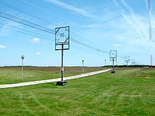
Single-wire line edit
Unbalanced lines were formerly much used for telegraph transmission, but this form of communication has now fallen into disuse. Cables are similar to twisted pair in that many cores are bundled into the same cable but only one conductor is provided per circuit and there is no twisting. All the circuits on the same route use a common path for the return current (earth return). There is a power transmission version of single-wire earth return in use in many locations.
General applications edit
Signal transfer edit
Electrical transmission lines are very widely used to transmit high frequency signals over long or short distances with minimum power loss. One familiar example is the down lead from a TV or radio aerial to the receiver.
Transmission line circuits edit
A large variety of circuits can also be constructed with transmission lines including impedance matching circuits, filters, power dividers and directional couplers.
Stepped transmission line edit

A stepped transmission line is used for broad range impedance matching. It can be considered as multiple transmission line segments connected in series, with the characteristic impedance of each individual element to be .[20] The input impedance can be obtained from the successive application of the chain relation


where is the wave number of the -th transmission line segment and is the length of this segment, and is the front-end impedance that loads the -th segment.


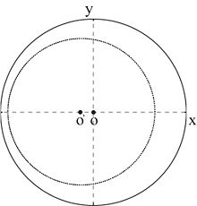


Because the characteristic impedance of each transmission line segment is often different from the impedance of the fourth, input cable (only shown as an arrow marked on the left side of the diagram above), the impedance transformation circle is off-centred along the axis of the Smith Chart whose impedance representation is usually normalized against .
Approximating lumped elements edit
At higher frequencies, the reactive parasitic effects of real world lumped elements, including inductors and capacitors, limits their usefulness.[21] Therefore, it is sometimes useful to approximate the electrical characteristics of inductors and capacitors with transmission lines at the higher frequencies using Richards' Transformations and then substitute the transmission lines for the lumped elements.[22][23]
More accurate forms of multimode high frequency inductor modeling with transmission lines exist for advanced designers.[24]
Stub filters edit
If a short-circuited or open-circuited transmission line is wired in parallel with a line used to transfer signals from point A to point B, then it will function as a filter. The method for making stubs is similar to the method for using Lecher lines for crude frequency measurement, but it is 'working backwards'. One method recommended in the RSGB's radiocommunication handbook is to take an open-circuited length of transmission line wired in parallel with the feeder delivering signals from an aerial. By cutting the free end of the transmission line, a minimum in the strength of the signal observed at a receiver can be found. At this stage the stub filter will reject this frequency and the odd harmonics, but if the free end of the stub is shorted then the stub will become a filter rejecting the even harmonics.
Wideband filters can be achieved using multiple stubs. However, this is a somewhat dated technique. Much more compact filters can be made with other methods such as parallel-line resonators.
Pulse generation edit
Transmission lines are used as pulse generators. By charging the transmission line and then discharging it into a resistive load, a rectangular pulse equal in length to twice the electrical length of the line can be obtained, although with half the voltage. A Blumlein transmission line is a related pulse forming device that overcomes this limitation. These are sometimes used as the pulsed power sources for radar transmitters and other devices.
Sound edit
The theory of sound wave propagation is very similar mathematically to that of electromagnetic waves, so techniques from transmission line theory are also used to build structures to conduct acoustic waves; and these are called acoustic transmission lines.
See also edit
References edit
Part of this article was derived from Federal Standard 1037C.
- ^ a b c Jackman, Shawn M.; Matt Swartz; Marcus Burton; Thomas W. Head (2011). CWDP Certified Wireless Design Professional Official Study Guide: Exam PW0-250. John Wiley & Sons. pp. Ch. 7. ISBN 978-1118041611.
- ^ a b Oklobdzija, Vojin G.; Ram K. Krishnamurthy (2006). High-Performance Energy-Efficient Microprocessor Design. Springer Science & Business Media. p. 297. ISBN 978-0387340470.
- ^ Guru, Bhag Singh; Hüseyin R. Hızıroğlu (2004). Electromagnetic Field Theory Fundamentals, 2nd Ed. Cambridge Univ. Press. pp. 422–423. ISBN 978-1139451925.
- ^ Schmitt, Ron Schmitt (2002). Electromagnetics Explained: A Handbook for Wireless/ RF, EMC, and High-Speed Electronics. Newnes. pp. 153. ISBN 978-0080505237.
- ^ Carr, Joseph J. (1997). Microwave & Wireless Communications Technology. USA: Newnes. pp. 46–47. ISBN 978-0750697071.
- ^ a b c Raisanen, Antti V.; Arto Lehto (2003). Radio Engineering for Wireless Communication and Sensor Applications. Artech House. pp. 35–37. ISBN 978-1580536691.
- ^ Weber, Ernst; Nebeker, Frederik (1994). The Evolution of Electrical Engineering. Piscataway, New Jersey: IEEE Press. ISBN 0-7803-1066-7.
- ^ a b Leon, Benjamin J.; Wintz, Paul A. (1970). Basic Linear Networks for Electrical and Electronics Engineer. US: Holt, Rinehart, and Winston. pp. 127 to 129. ISBN 0030783259.
{{cite book}}: CS1 maint: date and year (link) - ^ a b Pozar, David M. (2013). Microwave Engineering (4th ed.). Hoboken, NJ, US: John Wiley & Sones, Inc. pp. 174, 175. ISBN 978-81-265-4190-4.
{{cite book}}: CS1 maint: date and year (link) - ^ a b c Matthaei, George L.; Young, Leo; Jones, E. M. T. (1984). Microwave Filters, Impudence-Matching Networks, and Coupling Structures. 610 Washington Street, Dedham, Massachusetts, US: Artech House, Inc. (published 1985). p. 30. ISBN 0-89006-099-1.
{{cite book}}: CS1 maint: date and year (link) CS1 maint: location (link) - ^ a b Drakos, Nikos; Hennecke, Marcus; Moore, Ross; Swan, Herb (November 22, 2013). "Transmission Line". Quite Universal Circuit Simulator (Qucs).
{{cite web}}: CS1 maint: url-status (link) - ^ Pozar, David M. (1998). Microwave Engineering (2nd ed.). Canada: John Wiley & Sons, Inc. p. 192. ISBN 0-471-17096-8.
{{cite book}}: CS1 maint: date and year (link) - ^ University of Texas at Austin (December 14, 2015). "Microsoft Word - dissertation_def_rev.doc - ch_2.pdf" (PDF).
{{cite web}}: CS1 maint: url-status (link) - ^ "2.3: Scattering Parameters - Engineering LibreTexts". Engineering LibreTexts. October 21, 2020.
{{cite web}}: CS1 maint: url-status (link) - ^ Syed V. Ahamed, Victor B. Lawrence, Design and engineering of intelligent communication systems, pp.130–131, Springer, 1997 ISBN 0-7923-9870-X.
- ^ Evaluating Microphone Cable Performance & Specifications Archived 2016-05-09 at the Wayback Machine
- ^ How Starquad Works Archived 2016-11-12 at the Wayback Machine
- ^ Lampen, Stephen H. (2002). Audio/Video Cable Installer's Pocket Guide. McGraw-Hill. pp. 32, 110, 112. ISBN 978-0071386210.
- ^ Rayburn, Ray (2011). Eargle's The Microphone Book: From Mono to Stereo to Surround – A Guide to Microphone Design and Application (3 ed.). Focal Press. pp. 164–166. ISBN 978-0240820750.
- ^ Qian, Chunqi; Brey, William W. (2009). "Impedance matching with an adjustable segmented transmission line". Journal of Magnetic Resonance. 199 (1): 104–110. Bibcode:2009JMagR.199..104Q. doi:10.1016/j.jmr.2009.04.005. PMID 19406676.
- ^ "Microwaves101 | Parasitics". Microwave Encyclopedia. Retrieved April 2, 2024.
- ^ "2.12: Richards's Transformation - Engineering LibreTexts". Engineering LibreTexts. February 1, 2021.
- ^ Rhea, Randall W. (1995). HF Filter Design and Computer Simulation. McGraw-Hill, Inc. pp. 86–89. ISBN 0-07-052055-0.
{{cite book}}: CS1 maint: date and year (link) - ^ Rhea, Randall W. "A Multimode High-Frequency Inductor Model", Applied Microwaves & Wireless, November/December 1997, pp. 70-72, 74, 76-78, 80, Noble Publishing, Atlanta, Georgia, http://the-eye.unblocked2.us/public/Books/Electronic%20Archive/novdec1997-p70.pdf
- Steinmetz, Charles Proteus (27 August 1898). "The natural period of a transmission line and the frequency of lightning discharge therefrom". The Electrical World: 203–205.
- Grant, I.S.; Phillips, W.R. (1991-08-26). Electromagnetism (2nd ed.). John Wiley. ISBN 978-0-471-92712-9.
- Ulaby, F.T. (2004). Fundamentals of Applied Electromagnetics (2004 media ed.). Prentice Hall. ISBN 978-0-13-185089-7.
- "Chapter 17". Radio communication handbook. Radio Society of Great Britain. 1982. p. 20. ISBN 978-0-900612-58-9.
- Naredo, J.L.; Soudack, A.C.; Marti, J.R. (Jan 1995). "Simulation of transients on transmission lines with corona via the method of characteristics". IEE Proceedings - Generation, Transmission and Distribution. 142 (1): 81. doi:10.1049/ip-gtd:19951488. ISSN 1350-2360.
Further reading edit
- Honoring of Guglielmo Marconi. Annual Dinner of the Institute at the Waldorf-Astoria. New York: American Institute of Electrical Engineers. 13 January 1902.
- "Using Transmission Line Equations and Parameters". Star-Hspice Manual. Avant! Software. June 2001. Archived from the original on 25 September 2005.
- Cornille, P. (1990). "On the propagation of inhomogeneous waves". Journal of Physics D: Applied Physics. 23 (2): 129–135. Bibcode:1990JPhD...23..129C. doi:10.1088/0022-3727/23/2/001. S2CID 250788839.
- Farlow, S.J. (1982). Partial Differential Equations for Scientists and Engineers. J. Wiley and Sons. p. 126. ISBN 0-471-08639-8.
- Kupershmidt, Boris A. (1998). "Remarks on random evolutions in Hamiltonian representation". J. Nonlinear Math. Phys. 5 (4): 383–395. arXiv:math-ph/9810020. Bibcode:1998JNMP....5..483K. doi:10.2991/jnmp.1998.5.4.10. S2CID 14771417. Math-ph/9810020.
- "Transmission line matching". Department of Electronic and Information Engineering. High Frequency Circuit Design. Hong Kong Polytechnic University. EIE403. Archived from the original (PDF) on 2011-07-21. Retrieved 2005-09-24.
- Wilson, B. (19 October 2005). "Telegrapher's Equations". Connexions. Archived from the original on 9 January 2006.
- Wöhlbier, John Greaton (2000). Modeling and Analysis of a Traveling Wave under Multitone Excitation (PDF). Electrical and Computer Engineering (M.S.). Madison, WI: University of Wisconsin. §"Fundamental Equation" and §"Transforming the Telegrapher's Equations". Archived from the original (PDF) on 19 June 2006.
- "Wave Propagation along a Transmission Line" (Educational Java Applet). Educational Resources. Keysight Technologies.[permanent dead link] (May need to add "http://www.keysight.com" to your Java Exception Site list.)
- Qian, Chunqi; Brey, William W. (2009). "Impedance matching with an adjustable, segmented transmission line". Journal of Magnetic Resonance. 199 (1): 104–110. Bibcode:2009JMagR.199..104Q. doi:10.1016/j.jmr.2009.04.005. PMID 19406676.
External links edit
- "Transmission Line Calculator (Including radiation and surface-wave excitation losses)". terahertz.tudelft.nl. Delft, NL: Technical University of Delft.
- "Transmission Line Parameter Calculator". cecas.clemson.edu/cvel. Clemson, SC: Clemson University.