Trigonometric_integral Knowpia

In mathematics, trigonometric integrals are a family of nonelementary integrals involving trigonometric functions.

Integral cosine in the complex plane. Note the branch cut along the negative real axis.

Sine integral edit

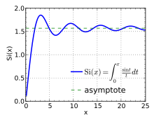
Plot of Si(x) for

0 \leq x \leq 8 π

.

Plot of the cosine integral function Ci(z) in the complex plane from −2 − 2i to 2 + 2i with colors created with Mathematica 13.1 function ComplexPlot3D

The different sine integral definitions are

\operatorname {Si} (x)=\int _{0}^{x}{\frac {\sin t}{t}}\,dt

\operatorname {si} (x)=-\int _{x}^{\infty }{\frac {\sin t}{t}}\,dt~.

Note that the integrand ${\frac {\sin(t)}{t}}$ is the sinc function, and also the zeroth spherical Bessel function. Since $sinc$ is an even entire function (holomorphic over the entire complex plane), $Si$ is entire, odd, and the integral in its definition can be taken along any path connecting the endpoints.

By definition, $Si(x)$ is the antiderivative of $sin x / x$ whose value is zero at $x = 0$ , and $si(x)$ is the antiderivative whose value is zero at $x = \infty$ . Their difference is given by the Dirichlet integral,

\operatorname {Si} (x)-\operatorname {si} (x)=\int _{0}^{\infty }{\frac {\sin t}{t}}\,dt={\frac {\pi }{2}}\quad {\text{ or }}\quad \operatorname {Si} (x)={\frac {\pi }{2}}+\operatorname {si} (x)~.

In signal processing, the oscillations of the sine integral cause overshoot and ringing artifacts when using the sinc filter, and frequency domain ringing if using a truncated sinc filter as a low-pass filter.

Related is the Gibbs phenomenon: If the sine integral is considered as the convolution of the sinc function with the heaviside step function, this corresponds to truncating the Fourier series, which is the cause of the Gibbs phenomenon.

Cosine integral edit

Plot of

Ci(x)

for 0 <

x

≤ 8

π

.

The different cosine integral definitions are

\operatorname {Cin} (x)=\int _{0}^{x}{\frac {1-\cos t}{t}}\,dt~,

\operatorname {Ci} (x)=-\int _{x}^{\infty }{\frac {\cos t}{t}}\,dt=\gamma +\ln x-\int _{0}^{x}{\frac {1-\cos t}{t}}\,dt\qquad ~{\text{ for }}~\left|\operatorname {Arg} (x)\right|<\pi ~,

where

γ \approx 0.57721566 ...

is the Euler–Mascheroni constant. Some texts use

ci

instead of

Ci

.

$Ci(x)$ is the antiderivative of $cos x / x$ (which vanishes as $x\to \infty$ ). The two definitions are related by

\operatorname {Ci} (x)=\gamma +\ln x-\operatorname {Cin} (x)~.

$Cin$ is an even, entire function. For that reason, some texts treat $Cin$ as the primary function, and derive $Ci$ in terms of $Cin$ .

Hyperbolic sine integral edit

The hyperbolic sine integral is defined as

\operatorname {Shi} (x)=\int _{0}^{x}{\frac {\sinh(t)}{t}}\,dt.

It is related to the ordinary sine integral by

\operatorname {Si} (ix)=i\operatorname {Shi} (x).

Hyperbolic cosine integral edit

The hyperbolic cosine integral is

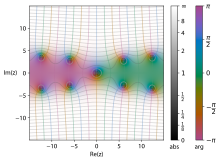
Plot of the hyperbolic cosine integral function Chi(z) in the complex plane from -2-2i to 2+2i with colors created with Mathematica 13.1 function ComplexPlot3D

\operatorname {Chi} (x)=\gamma +\ln x+\int _{0}^{x}{\frac {\cosh t-1}{t}}\,dt\qquad ~{\text{ for }}~\left|\operatorname {Arg} (x)\right|<\pi ~,

where

\gamma

is the Euler–Mascheroni constant.

It has the series expansion

\operatorname {Chi} (x)=\gamma +\ln(x)+{\frac {x^{2}}{4}}+{\frac {x^{4}}{96}}+{\frac {x^{6}}{4320}}+{\frac {x^{8}}{322560}}+{\frac {x^{10}}{36288000}}+O(x^{12}).

Auxiliary functions edit

Trigonometric integrals can be understood in terms of the so-called "auxiliary functions"

{\begin{array}{rcl}f(x)&\equiv &\int _{0}^{\infty }{\frac {\sin(t)}{t+x}}\,dt&=&\int _{0}^{\infty }{\frac {e^{-xt}}{t^{2}+1}}\,dt&=&\operatorname {Ci} (x)\sin(x)+\left[{\frac {\pi }{2}}-\operatorname {Si} (x)\right]\cos(x)~,\\g(x)&\equiv &\int _{0}^{\infty }{\frac {\cos(t)}{t+x}}\,dt&=&\int _{0}^{\infty }{\frac {te^{-xt}}{t^{2}+1}}\,dt&=&-\operatorname {Ci} (x)\cos(x)+\left[{\frac {\pi }{2}}-\operatorname {Si} (x)\right]\sin(x)~.\end{array}}

Using these functions, the trigonometric integrals may be re-expressed as (cf. Abramowitz & Stegun, p. 232)

{\begin{array}{rcl}{\frac {\pi }{2}}-\operatorname {Si} (x)=-\operatorname {si} (x)&=&f(x)\cos(x)+g(x)\sin(x)~,\qquad {\text{ and }}\\\operatorname {Ci} (x)&=&f(x)\sin(x)-g(x)\cos(x)~.\\\end{array}}

Nielsen's spiral edit

Nielsen's spiral.

The spiral formed by parametric plot of $si , ci$ is known as Nielsen's spiral.

x(t)=a\times \operatorname {ci} (t)

y(t)=a\times \operatorname {si} (t)

The spiral is closely related to the Fresnel integrals and the Euler spiral. Nielsen's spiral has applications in vision processing, road and track construction and other areas.^[1]

Expansion edit

Various expansions can be used for evaluation of trigonometric integrals, depending on the range of the argument.

Asymptotic series (for large argument) edit

\operatorname {Si} (x)\sim {\frac {\pi }{2}}-{\frac {\cos x}{x}}\left(1-{\frac {2!}{x^{2}}}+{\frac {4!}{x^{4}}}-{\frac {6!}{x^{6}}}\cdots \right)-{\frac {\sin x}{x}}\left({\frac {1}{x}}-{\frac {3!}{x^{3}}}+{\frac {5!}{x^{5}}}-{\frac {7!}{x^{7}}}\cdots \right)

\operatorname {Ci} (x)\sim {\frac {\sin x}{x}}\left(1-{\frac {2!}{x^{2}}}+{\frac {4!}{x^{4}}}-{\frac {6!}{x^{6}}}\cdots \right)-{\frac {\cos x}{x}}\left({\frac {1}{x}}-{\frac {3!}{x^{3}}}+{\frac {5!}{x^{5}}}-{\frac {7!}{x^{7}}}\cdots \right)~.

These series are asymptotic and divergent, although can be used for estimates and even precise evaluation at $ℜ(x) ≫ 1$ .

Convergent series edit

\operatorname {Si} (x)=\sum _{n=0}^{\infty }{\frac {(-1)^{n}x^{2n+1}}{(2n+1)(2n+1)!}}=x-{\frac {x^{3}}{3!\cdot 3}}+{\frac {x^{5}}{5!\cdot 5}}-{\frac {x^{7}}{7!\cdot 7}}\pm \cdots

\operatorname {Ci} (x)=\gamma +\ln x+\sum _{n=1}^{\infty }{\frac {(-1)^{n}x^{2n}}{2n(2n)!}}=\gamma +\ln x-{\frac {x^{2}}{2!\cdot 2}}+{\frac {x^{4}}{4!\cdot 4}}\mp \cdots

These series are convergent at any complex $x$ , although for $| x | ≫ 1$ , the series will converge slowly initially, requiring many terms for high precision.

Derivation of series expansion edit

From the Maclaurin series expansion of sine:

\sin \,x=x-{\frac {x^{3}}{3!}}+{\frac {x^{5}}{5!}}-{\frac {x^{7}}{7!}}+{\frac {x^{9}}{9!}}-{\frac {x^{11}}{11!}}+\cdots

{\frac {\sin \,x}{x}}=1-{\frac {x^{2}}{3!}}+{\frac {x^{4}}{5!}}-{\frac {x^{6}}{7!}}+{\frac {x^{8}}{9!}}-{\frac {x^{10}}{11!}}+\cdots

\therefore \int {\frac {\sin \,x}{x}}dx=x-{\frac {x^{3}}{3!\cdot 3}}+{\frac {x^{5}}{5!\cdot 5}}-{\frac {x^{7}}{7!\cdot 7}}+{\frac {x^{9}}{9!\cdot 9}}-{\frac {x^{11}}{11!\cdot 11}}+\cdots

Relation with the exponential integral of imaginary argument edit

The function

\operatorname {E} _{1}(z)=\int _{1}^{\infty }{\frac {\exp(-zt)}{t}}\,dt\qquad ~{\text{ for }}~\Re (z)\geq 0

is called the exponential integral. It is closely related to

Si

and

Ci

,

\operatorname {E} _{1}(ix)=i\left(-{\frac {\pi }{2}}+\operatorname {Si} (x)\right)-\operatorname {Ci} (x)=i\operatorname {si} (x)-\operatorname {ci} (x)\qquad ~{\text{ for }}~x>0~.

As each respective function is analytic except for the cut at negative values of the argument, the area of validity of the relation should be extended to (Outside this range, additional terms which are integer factors of $π$ appear in the expression.)

Cases of imaginary argument of the generalized integro-exponential function are

\int _{1}^{\infty }\cos(ax){\frac {\ln x}{x}}\,dx=-{\frac {\pi ^{2}}{24}}+\gamma \left({\frac {\gamma }{2}}+\ln a\right)+{\frac {\ln ^{2}a}{2}}+\sum _{n\geq 1}{\frac {(-a^{2})^{n}}{(2n)!(2n)^{2}}}~,

which is the real part of

\int _{1}^{\infty }e^{iax}{\frac {\ln x}{x}}\,dx=-{\frac {\pi ^{2}}{24}}+\gamma \left({\frac {\gamma }{2}}+\ln a\right)+{\frac {\ln ^{2}a}{2}}-{\frac {\pi }{2}}i\left(\gamma +\ln a\right)+\sum _{n\geq 1}{\frac {(ia)^{n}}{n!n^{2}}}~.

Similarly

\int _{1}^{\infty }e^{iax}{\frac {\ln x}{x^{2}}}\,dx=1+ia\left[-{\frac {\pi ^{2}}{24}}+\gamma \left({\frac {\gamma }{2}}+\ln a-1\right)+{\frac {\ln ^{2}a}{2}}-\ln a+1\right]+{\frac {\pi a}{2}}{\Bigl (}\gamma +\ln a-1{\Bigr )}+\sum _{n\geq 1}{\frac {(ia)^{n+1}}{(n+1)!n^{2}}}~.

Efficient evaluation edit

Padé approximants of the convergent Taylor series provide an efficient way to evaluate the functions for small arguments. The following formulae, given by Rowe et al. (2015),^[2] are accurate to better than $10 -16$ for $0 \leq x \leq 4$ ,

{\begin{array}{rcl}\operatorname {Si} (x)&\approx &x\cdot \left({\frac {\begin{array}{l}1-4.54393409816329991\cdot 10^{-2}\cdot x^{2}+1.15457225751016682\cdot 10^{-3}\cdot x^{4}-1.41018536821330254\cdot 10^{-5}\cdot x^{6}\\~~~+9.43280809438713025\cdot 10^{-8}\cdot x^{8}-3.53201978997168357\cdot 10^{-10}\cdot x^{10}+7.08240282274875911\cdot 10^{-13}\cdot x^{12}\\~~~-6.05338212010422477\cdot 10^{-16}\cdot x^{14}\end{array}}{\begin{array}{l}1+1.01162145739225565\cdot 10^{-2}\cdot x^{2}+4.99175116169755106\cdot 10^{-5}\cdot x^{4}+1.55654986308745614\cdot 10^{-7}\cdot x^{6}\\~~~+3.28067571055789734\cdot 10^{-10}\cdot x^{8}+4.5049097575386581\cdot 10^{-13}\cdot x^{10}+3.21107051193712168\cdot 10^{-16}\cdot x^{12}\end{array}}}\right)\\&~&\\\operatorname {Ci} (x)&\approx &\gamma +\ln(x)+\\&&x^{2}\cdot \left({\frac {\begin{array}{l}-0.25+7.51851524438898291\cdot 10^{-3}\cdot x^{2}-1.27528342240267686\cdot 10^{-4}\cdot x^{4}+1.05297363846239184\cdot 10^{-6}\cdot x^{6}\\~~~-4.68889508144848019\cdot 10^{-9}\cdot x^{8}+1.06480802891189243\cdot 10^{-11}\cdot x^{10}-9.93728488857585407\cdot 10^{-15}\cdot x^{12}\\\end{array}}{\begin{array}{l}1+1.1592605689110735\cdot 10^{-2}\cdot x^{2}+6.72126800814254432\cdot 10^{-5}\cdot x^{4}+2.55533277086129636\cdot 10^{-7}\cdot x^{6}\\~~~+6.97071295760958946\cdot 10^{-10}\cdot x^{8}+1.38536352772778619\cdot 10^{-12}\cdot x^{10}+1.89106054713059759\cdot 10^{-15}\cdot x^{12}\\~~~+1.39759616731376855\cdot 10^{-18}\cdot x^{14}\\\end{array}}}\right)\end{array}}

The integrals may be evaluated indirectly via auxiliary functions $f(x)$ and $g(x)$ , which are defined by

$\operatorname {Si} (x)={\frac {\pi }{2}}-f(x)\cos(x)-g(x)\sin(x)$		$\operatorname {Ci} (x)=f(x)\sin(x)-g(x)\cos(x)$
or equivalently
$f(x)\equiv \left[{\frac {\pi }{2}}-\operatorname {Si} (x)\right]\cos(x)+\operatorname {Ci} (x)\sin(x)$		$g(x)\equiv \left[{\frac {\pi }{2}}-\operatorname {Si} (x)\right]\sin(x)-\operatorname {Ci} (x)\cos(x)$

For $x\geq 4$ the Padé rational functions given below approximate $f(x)$ and $g(x)$ with error less than 10⁻¹⁶:^[2]

{\begin{array}{rcl}f(x)&\approx &{\dfrac {1}{x}}\cdot \left({\frac {\begin{array}{l}1+7.44437068161936700618\cdot 10^{2}\cdot x^{-2}+1.96396372895146869801\cdot 10^{5}\cdot x^{-4}+2.37750310125431834034\cdot 10^{7}\cdot x^{-6}\\~~~+1.43073403821274636888\cdot 10^{9}\cdot x^{-8}+4.33736238870432522765\cdot 10^{10}\cdot x^{-10}+6.40533830574022022911\cdot 10^{11}\cdot x^{-12}\\~~~+4.20968180571076940208\cdot 10^{12}\cdot x^{-14}+1.00795182980368574617\cdot 10^{13}\cdot x^{-16}+4.94816688199951963482\cdot 10^{12}\cdot x^{-18}\\~~~-4.94701168645415959931\cdot 10^{11}\cdot x^{-20}\end{array}}{\begin{array}{l}1+7.46437068161927678031\cdot 10^{2}\cdot x^{-2}+1.97865247031583951450\cdot 10^{5}\cdot x^{-4}+2.41535670165126845144\cdot 10^{7}\cdot x^{-6}\\~~~+1.47478952192985464958\cdot 10^{9}\cdot x^{-8}+4.58595115847765779830\cdot 10^{10}\cdot x^{-10}+7.08501308149515401563\cdot 10^{11}\cdot x^{-12}\\~~~+5.06084464593475076774\cdot 10^{12}\cdot x^{-14}+1.43468549171581016479\cdot 10^{13}\cdot x^{-16}+1.11535493509914254097\cdot 10^{13}\cdot x^{-18}\end{array}}}\right)\\&&\\g(x)&\approx &{\dfrac {1}{x^{2}}}\cdot \left({\frac {\begin{array}{l}1+8.1359520115168615\cdot 10^{2}\cdot x^{-2}+2.35239181626478200\cdot 10^{5}\cdot x^{-4}+3.12557570795778731\cdot 10^{7}\cdot x^{-6}\\~~~+2.06297595146763354\cdot 10^{9}\cdot x^{-8}+6.83052205423625007\cdot 10^{10}\cdot x^{-10}+1.09049528450362786\cdot 10^{12}\cdot x^{-12}\\~~~+7.57664583257834349\cdot 10^{12}\cdot x^{-14}+1.81004487464664575\cdot 10^{13}\cdot x^{-16}+6.43291613143049485\cdot 10^{12}\cdot x^{-18}\\~~~-1.36517137670871689\cdot 10^{12}\cdot x^{-20}\end{array}}{\begin{array}{l}1+8.19595201151451564\cdot 10^{2}\cdot x^{-2}+2.40036752835578777\cdot 10^{5}\cdot x^{-4}+3.26026661647090822\cdot 10^{7}\cdot x^{-6}\\~~~+2.23355543278099360\cdot 10^{9}\cdot x^{-8}+7.87465017341829930\cdot 10^{10}\cdot x^{-10}+1.39866710696414565\cdot 10^{12}\cdot x^{-12}\\~~~+1.17164723371736605\cdot 10^{13}\cdot x^{-14}+4.01839087307656620\cdot 10^{13}\cdot x^{-16}+3.99653257887490811\cdot 10^{13}\cdot x^{-18}\end{array}}}\right)\\\end{array}}

References edit

^ Gray (1993). Modern Differential Geometry of Curves and Surfaces. Boca Raton. p. 119.{{cite book}}: CS1 maint: location missing publisher (link)
^ ^a ^b Rowe, B.; et al. (2015). "GALSIM: The modular galaxy image simulation toolkit". Astronomy and Computing. 10: 121. arXiv:1407.7676. Bibcode:2015A&C....10..121R. doi:10.1016/j.ascom.2015.02.002. S2CID 62709903.

Abramowitz, Milton; Stegun, Irene Ann, eds. (1983) [June 1964]. "Chapter 5". Handbook of Mathematical Functions with Formulas, Graphs, and Mathematical Tables. Applied Mathematics Series. Vol. 55 (Ninth reprint with additional corrections of tenth original printing with corrections (December 1972); first ed.). Washington D.C.; New York: United States Department of Commerce, National Bureau of Standards; Dover Publications. p. 231. ISBN 978-0-486-61272-0. LCCN 64-60036. MR 0167642. LCCN 65-12253.