


Summary
The computer graphics pipeline, also known as the rendering pipeline or graphics pipeline, is a framework within computer graphics that outlines the necessary procedures for transforming a three-dimensional (3D) scene into a two-dimensional (2D) representation on a screen.[1] Once a 3D model is generated, the graphics pipeline converts the model into a visually perceivable format on the computer display.[2] Due to the dependence on specific software, hardware configurations, and desired display attributes, a universally applicable graphics pipeline does not exist. Nevertheless, graphics application programming interfaces (APIs), such as Direct3D, OpenGL and Vulkan were developed to standardize common procedures and oversee the graphics pipeline of a given hardware accelerator. These APIs provide an abstraction layer over the underlying hardware, relieving programmers from the need to write code explicitly targeting various graphics hardware accelerators like AMD, Intel, Nvidia, and others.
The model of the graphics pipeline is usually used in real-time rendering. Often, most of the pipeline steps are implemented in hardware, which allows for special optimizations. The term "pipeline" is used in a similar sense for the pipeline in processors: the individual steps of the pipeline run in parallel as long as any given step has what it needs.
Concept edit
The 3D pipeline usually refers to the most common form of computer 3D rendering called 3D polygon rendering[citation needed], distinct from Raytracing and Raycasting. In Raycasting, a ray originates at the point where the camera resides, and if that ray hits a surface, the color and lighting of the point on the surface where the ray hit is calculated. In 3D polygon rendering the reverse happens- the area that is in view of the camera is calculated and then rays are created from every part of every surface in view of the camera and traced back to the camera.[3]
Structure edit
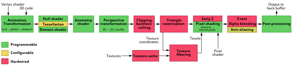
A graphics pipeline can be divided into three main parts: Application, Geometry and Rasterization.[4]

Application edit
The application step is executed by the software on the main processor (CPU). During the application step, changes are made to the scene as required, for example, by user interaction by means of input devices or during an animation. The new scene with all its primitives, usually triangles, lines and points, is then passed on to the next step in the pipeline.
Examples of tasks that are typically done in the application step are collision detection, animation, morphing, and acceleration techniques using spatial subdivision schemes such as Quadtrees or Octrees. These are also used to reduce the amount of main memory required at a given time. The "world" of a modern computer game is far larger than what could fit into memory at once.
Geometry edit
The geometry step (with Geometry pipeline), which is responsible for the majority of the operations with polygons and their vertices (with Vertex pipeline), can be divided into the following five tasks. It depends on the particular implementation of how these tasks are organized as actual parallel pipeline steps.

Definitions edit
A vertex (plural: vertices) is a point in the world. Many points are used to join the surfaces. In special cases, point clouds are drawn directly, but this is still the exception.
A triangle is the most common geometric primitive of computer graphics. It is defined by its three vertices and a normal vector - the normal vector serves to indicate the front face of the triangle and is a vector that is perpendicular to the surface. The triangle may be provided with a color or with a texture (image "glued" on top of it). Triangles are preferred over rectangles because their three points always exist in a single plane.
The World Coordinate System edit
The world coordinate system is the coordinate system in which the virtual world is created. This should meet a few conditions for the following mathematics to be easily applicable:
- It must be a rectangular Cartesian coordinate system in which all axes are equally scaled.
How the unit of the coordinate system is defined, is left to the developer. Whether, therefore, the unit vector of the system is to correspond in reality to one meter or an Ångström depends on the application.
- Whether a right-handed or a left-handed coordinate system is to be used may be determined by the graphic library to be used.
- Example: If we are to develop a flight simulator, we can choose the world coordinate system so that the origin is in the middle of the Earth and the unit is set to one meter. In addition, in order to make the reference to reality easier, we define that the X axis should intersect the equator on the zero meridian, and the Z axis passes through the poles. In a Right-handed system, the Y-axis runs through the 90°-East meridian (somewhere in the Indian Ocean). Now we have a coordinate system that describes every point on Earth in three-dimensional Cartesian coordinates. In this coordinate system, we are now modeling the principles of our world, mountains, valleys and oceans.
- Note: Aside from computer geometry, geographic coordinates are used for the Earth, i.e., latitude and longitude, as well as altitudes above sea level. The approximate conversion - if one does not consider the fact that the Earth is not an exact sphere - is simple:
- with R = Radius of the Earth [6.378.137m], lat = Latitude, long = Longitude, hasl = height above sea level.
- All of the following examples apply in a right-handed system. For a left-handed system the signs may need to be interchanged.

The objects contained within the scene (houses, trees, cars) are often designed in their own object coordinate system (also called model coordinate system or local coordinate system) for reasons of simpler modeling. To assign these objects to coordinates in the world coordinate system or global coordinate system of the entire scene, the object coordinates are transformed by means of translation, rotation or scaling. This is done by multiplying the corresponding transformation matrices. In addition, several differently transformed copies can be formed from one object, for example a forest from a tree; This technique is called instancing.
- In order to place a model of an aircraft in the world, we first determine four matrices. Since we work in three-dimensional space, we need four-dimensional homogeneous matrices for our calculations.
First, we need three rotation matrices, namely one for each of the three aircraft axes (vertical axis, transverse axis, longitudinal axis).
- Around the X axis (usually defined as a longitudinal axis in the object coordinate system)

- Around the Y axis (usually defined as the transverse axis in the object coordinate system)

- Around the Z axis (usually defined as vertical axis in the object coordinate system)

We also use a translation matrix that moves the aircraft to the desired point in our world: .

- Remark: The above matrices are transposed with respect to the ones in the article rotation matrix. See further down for an explanation why.
Now we could calculate the position of the vertices of the aircraft in world coordinates by multiplying each point successively with these four matrices. Since the multiplication of a matrix with a vector is quite expensive (time-consuming), one usually takes another path and first multiplies the four matrices together. The multiplication of two matrices is even more expensive, but must be executed only once for the whole object. The multiplications and are equivalent. Thereafter, the resulting matrix could be applied to the vertices. In practice, however, the multiplication with the vertices is still not applied, but the camera matrices (see below) are determined first.


- For our example from above, however, the translation has to be determined somewhat differently, since the common meaning of up - apart from at the North Pole - does not coincide with our definition of the positive Z axis and therefore the model must also be rotated around the center of the Earth: The first step pushes the origin of the model to the correct height above the Earth's surface, then it is rotated by latitude and longitude.

The order in which the matrices are applied is important, because the matrix multiplication is not commutative. This also applies to the three rotations, which can be demonstrated by an example: The point (1, 0, 0) lies on the X-axis, if one rotates it first by 90° around the X- and then around The Y-axis, it ends up on the Z-axis (the rotation around the X-axis has no effect on a point that is on the axis). If, on the other hand, one rotates around the Y-axis first and then around the X-axis, the resulting point is located on the Y-axis. The sequence itself is arbitrary as long as it is always the same. The sequence with x, then y, then z (roll, pitch, heading) is often the most intuitive, because the rotation causes the compass direction to coincide with the direction of the "nose".
There are also two conventions to define these matrices, depending on whether you want to work with column vectors or row vectors. Different graphics libraries have different preferences here. OpenGL prefers column vectors, DirectX row vectors. The decision determines from which side the point vectors are to be multiplied by the transformation matrices. For column vectors, the multiplication is performed from the right, i.e. , where vout and vin are 4x1 column vectors. The concatenation of the matrices also is done from the right to left, i.e., for example , when first rotating and then shifting.


In the case of row vectors, this works exactly the other way round. The multiplication now takes place from left as with 1x4-row vectors and the concatenation is when we also first rotate and then move. The matrices shown above are valid for the second case, while those for column vectors are transposed. The rule [5] applies, which for multiplication with vectors means that you can switch the multiplication order by transposing the matrix.


In matrix chaining, each transformation defines a new coordinate system, allowing for flexible extensions. For instance, an aircraft's propeller, modeled separately, can be attached to the aircraft nose through translation, which only shifts from the model to the propeller coordinate system. To render the aircraft, its transformation matrix is first computed to transform the points, followed by multiplying the propeller model matrix to the aircraft's matrix for the propeller points. This calculated matrix is known as the 'world matrix,' essential for each object in the scene before rendering. The application can then dynamically alter these matrices, such as updating the aircraft's position with each frame based on speed.
The matrix calculated in this way is also called the world matrix. It must be determined for each object in the world before rendering. The application can introduce changes here, for example change the position of the aircraft according to the speed after each frame.
Camera Transformation edit
In addition to the objects, the scene also defines a virtual camera or viewer that indicates the position and direction of view relative to which the scene is rendered. The scene is transformed so that the camera is at the origin looking along the Z axis. The resulting coordinate system is called the camera coordinate system and the transformation is called camera transformation or View Transformation.
- The view matrix is usually determined from camera position, target point (where the camera looks) and an "up vector" ("up" from the viewer's viewpoint). First three auxiliary vectors are required:
Zaxis = normal(cameraPosition - cameraTarget)Xaxis = normal(cross(cameraUpVector, Zaxis))Yaxis = cross(Zaxis, Xaxis )- With normal(v) = normalization of the vector v;
- cross(v1, v2) = cross product of v1 and v2.
- Finally, the matrix:
- with dot(v1, v2) = dot product of v1 and v2.

Projection edit
The 3D projection step transforms the view volume into a cube with the corner point coordinates (-1, -1, 0) and (1, 1, 1); Occasionally other target volumes are also used. This step is called projection, even though it transforms a volume into another volume, since the resulting Z coordinates are not stored in the image, but are only used in Z-buffering in the later rastering step. In a perspective illustration, a central projection is used. To limit the number of displayed objects, two additional clipping planes are used; The visual volume is therefore a truncated pyramid (frustum). The parallel or orthogonal projection is used, for example, for technical representations because it has the advantage that all parallels in the object space are also parallel in the image space, and the surfaces and volumes are the same size regardless of the distance from the viewer. Maps use, for example, an orthogonal projection (so-called orthophoto), but oblique images of a landscape cannot be used in this way - although they can technically be rendered, they seem so distorted that we cannot make any use of them. The formula for calculating a perspective mapping matrix is:

- With h = cot (fieldOfView / 2.0) (aperture angle of the camera); w = h / aspect Ratio (aspect ratio of the target image); near = Smallest distance to be visible; far = The longest distance to be visible.
The reasons why the smallest and the greatest distance have to be given here are, on the one hand, that this distance is divided by in order to reach the scaling of the scene (more distant objects are smaller in a perspective image than near objects), and on the other hand to scale the Z values to the range 0..1, for filling the Z-buffer. This buffer often has only a resolution of 16 bits, which is why the near and far values should be chosen carefully. A too large difference between the near and the far value leads to so-called Z-fighting because of the low resolution of the Z-buffer. It can also be seen from the formula that the near value cannot be 0, because this point is the focus point of the projection. There is no picture at this point.
For the sake of completeness, the formula for parallel projection (orthogonal projection):

- with w = width of the target cube (dimension in units of the world coordinate system); H = w / aspect Ratio (aspect ratio of the target image); near = Smallest distance to be visible; far = The longest distance to be visible.
For reasons of efficiency, the camera and projection matrix are usually combined into a transformation matrix so that the camera coordinate system is omitted. The resulting matrix is usually the same for a single image, while the world matrix looks different for each object. In practice, therefore, view and projection are pre-calculated so that only the world matrix has to be adapted during the display. However, more complex transformations such as vertex blending are possible. Freely programmable geometry shaders that modify the geometry can also be executed.
In the actual rendering step, the world matrix * camera matrix * projection matrix is calculated and then finally applied to every single point. Thus, the points of all objects are transferred directly to the screen coordinate system (at least almost, the value range of the axes are still -1..1 for the visible range, see section "Window-Viewport-Transformation").
Lighting edit
Often a scene contains light sources placed at different positions to make the lighting of the objects appear more realistic. In this case, a gain factor for the texture is calculated for each vertex based on the light sources and the material properties associated with the corresponding triangle. In the later rasterization step, the vertex values of a triangle are interpolated over its surface. A general lighting (ambient light) is applied to all surfaces. It is the diffuse and thus direction-independent brightness of the scene. The sun is a directed light source, which can be assumed to be infinitely far away. The illumination effected by the sun on a surface is determined by forming the scalar product of the directional vector from the sun and the normal vector of the surface. If the value is negative, the surface is facing the sun.
Clipping edit


Only the primitives which are within the visual volume need to actually be rastered (drawn). This visual volume is defined as the inside of a frustum, a shape in the form of a pyramid with a cut off top. Primitives which are completely outside the visual volume are discarded; This is called frustum culling. Further culling methods such as back face culling, which reduce the number of primitives to be considered, can theoretically be executed in any step of the graphics pipeline. Primitives which are only partially inside the cube must be clipped against the cube. The advantage of the previous projection step is that the clipping always takes place against the same cube. Only the - possibly clipped - primitives, which are within the visual volume, are forwarded to the final step.
Window-Viewport transformation edit

In order to output the image to any target area (viewport) of the screen, another transformation, the Window-Viewport transformation, must be applied. This is a shift, followed by scaling. The resulting coordinates are the device coordinates of the output device. The viewport contains 6 values: height and width of the window in pixels, the upper left corner of the window in window coordinates (usually 0, 0) and the minimum and maximum values for Z (usually 0 and 1).
- Formally:
- With vp=Viewport; v=Point after projection

On modern hardware, most of the geometry computation steps are performed in the vertex shader. This is, in principle, freely programmable, but generally performs at least the transformation of the points and the illumination calculation. For the DirectX programming interface, the use of a custom vertex shader is necessary from version 10, while older versions still have a standard shader.
Rasterization edit
The rasterization step is the final step before the fragment shader pipeline that all primitives are rasterized with. In the rasterization step, discrete fragments are created from continuous primitives.
In this stage of the graphics pipeline, the grid points are also called fragments, for the sake of greater distinctiveness. Each fragment corresponds to one pixel in the frame buffer and this corresponds to one pixel of the screen. These can be colored (and possibly illuminated). Furthermore, it is necessary to determine the visible, closer to the observer fragment, in the case of overlapping polygons. A Z-buffer is usually used for this so-called hidden surface determination. The color of a fragment depends on the illumination, texture, and other material properties of the visible primitive and is often interpolated using the triangle vertex properties. Where available, a fragment shader (also called Pixel Shader) is run in the rastering step for each fragment of the object. If a fragment is visible, it can now be mixed with already existing color values in the image if transparency or multi-sampling is used. In this step, one or more fragments become a pixel.
To prevent that the user sees the gradual rasterization of the primitives, double buffering takes place. The rasterization is carried out in a special memory area. Once the image has been completely rasterized, it is copied to the visible area of the image memory.
Inverse edit
All matrices used are nonsingular and thus invertible. Since the multiplication of two nonsingular matrices creates another nonsingular matrix, the entire transformation matrix is also invertible. The inverse is required to recalculate world coordinates from screen coordinates - for example, to determine from the mouse pointer position the clicked object. However, since the screen and the mouse have only two dimensions, the third is unknown. Therefore, a ray is projected at the cursor position into the world and then the intersection of this ray with the polygons in the world is determined.
Shader edit
Classic graphics cards are still relatively close to the graphics pipeline. With increasing demands on the GPU, restrictions were gradually removed to create more flexibility. Modern graphics cards use a freely programmable, shader-controlled pipeline, which allows direct access to individual processing steps. To relieve the main processor, additional processing steps have been moved to the pipeline and the GPU.
The most important shader units are vertex shaders, geometry shaders, and pixel shaders.
The Unified Shader has been introduced to take full advantage of all units. This gives a single large pool of shader units. As required, the pool is divided into different groups of shaders. A strict separation between the shader types is therefore no longer useful.
It is also possible to use a so-called compute-shader to perform any calculations off the display of a graphic on the GPU. The advantage is that they run very parallel, but there are limitations. These universal calculations are also called general-purpose computing on graphics processing units, or GPGPU for short.
Mesh shaders are a recent addition, aim to overcome the bottlenecks of the geometry pipeline fixed layout.[6]
See also edit
Sources edit
- Akenine-Möller, Tomas; Haines, Eric; Hoffman, Naty (2019) [2008]. Real-Time Rendering. CRC Press. ISBN 9781315362007.
- Bender, Michael; Brill, Manfred (2006). Computergrafik: ein anwendungsorientiertes Lehrbuch. München: Hanser. ISBN 3-446-40434-1.
- Fischer, Martin (2011-07-04). Pixel-Fabrik. Wie Grafikchips Spielewelten auf den Schirm zaubern. c't Magazin für Computer Technik. Heise Zeitschriften Verlag. p. 180. ISSN 0724-8679.
References edit
- ^ "Graphics Pipeline". Microsoft. May 30, 2018. Retrieved 15 June 2015.
- ^ "Lecture: Graphics pipeline and animation". Archived from the original on 7 December 2017. Retrieved 15 June 2015.
- ^ Lawrence, Jason (October 22, 2012). "3D Polygon Rendering Pipeline" (PDF). Archived (PDF) from the original on December 29, 2016. Retrieved 2019-09-19.
- ^ Akenine-Möller, Haines & Hoffman 2019, p. 13 2.1 Architecture Figure 2.2
- ^ Nipp, K.; Stoffer, D. (1998). Lineare Algebra. v/d/f Hochschulverlag der ETH Zürich. ISBN 3-7281-2649-7.
- ^ Advanced API Performance: Mesh Shaders
External links edit
- [dead link]