The result ${\displaystyle x}$  of some experiment has two possible explanations – hypotheses ${\displaystyle H_{0}}$  and ${\displaystyle H_{1}}$  – and some prior distribution ${\displaystyle \pi }$  representing uncertainty as to which hypothesis is more accurate before taking into account ${\displaystyle x}$ .

Lindley's paradox occurs when

1. The result ${\displaystyle x}$  is "significant" by a frequentist test of ${\displaystyle H_{0},}$  indicating sufficient evidence to reject ${\displaystyle H_{0},}$  say, at the 5% level, and
2. The posterior probability of ${\displaystyle H_{0}}$  given ${\displaystyle x}$  is high, indicating strong evidence that ${\displaystyle H_{0}}$  is in better agreement with ${\displaystyle x}$  than ${\displaystyle H_{1}.}$ 

These results can occur at the same time when ${\displaystyle H_{0}}$  is very specific, ${\displaystyle H_{1}}$  more diffuse, and the prior distribution does not strongly favor one or the other, as seen below.

The following numerical example illustrates Lindley's paradox. In a certain city 49,581 boys and 48,870 girls have been born over a certain time period. The observed proportion ${\displaystyle x}$  of male births is thus 49581/98451 ≈ 0.5036. We assume the fraction of male births is a binomial variable with parameter ${\displaystyle \theta .}$  We are interested in testing whether ${\displaystyle \theta }$  is 0.5 or some other value. That is, our null hypothesis is ${\displaystyle H_{0}:\theta =0.5,}$  and the alternative is ${\displaystyle H_{1}:\theta \neq 0.5.}$ 

Frequentist approach edit

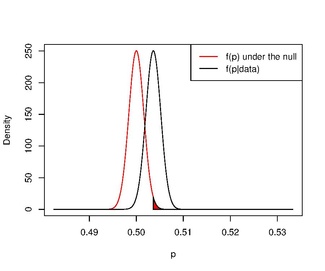
The frequentist approach to testing ${\displaystyle H_{0}}$  is to compute a p-value, the probability of observing a fraction of boys at least as large as ${\displaystyle x}$  assuming ${\displaystyle H_{0}}$  is true. Because the number of births is very large, we can use a normal approximation for the fraction of male births ${\displaystyle X\sim N(\mu ,\sigma ^{2}),}$  with ${\displaystyle \mu =np=n\theta =98\,451\times 0.5=49\,225.5}$  and ${\displaystyle \sigma ^{2}=n\theta (1-\theta )=98\,451\times 0.5\times 0.5=24\,612.75,}$  to compute

${\displaystyle {\begin{aligned}P(X\geq x\mid \mu =49\,225.5)=\int _{x=49\,581}^{98\,451}{\frac {1}{\sqrt {2\pi \sigma ^{2}}}}e^{-{\frac {1}{2}}\left({\frac {u-\mu }{\sigma }}\right)^{2}}\,du\\=\int _{x=49\,581}^{98\,451}{\frac {1}{\sqrt {2\pi (24\,612.75)}}}e^{-{\frac {(u-49\,225.5)^{2}}{2\times 24\,612.75}}}\,du\approx 0.0117.\end{aligned}}}$ 

We would have been equally surprised if we had seen 49581 female births, i.e. ${\displaystyle x\approx 0.4964,}$  so a frequentist would usually perform a two-sided test, for which the p-value would be ${\displaystyle p\approx 2\times 0.0117=0.0235.}$  In both cases, the p-value is lower than the significance level α = 5%, so the frequentist approach rejects ${\displaystyle H_{0},}$  as it disagrees with the observed data.

Bayesian approach edit

Assuming no reason to favor one hypothesis over the other, the Bayesian approach would be to assign prior probabilities ${\displaystyle \pi (H_{0})=\pi (H_{1})=0.5}$  and a uniform distribution to ${\displaystyle \theta }$  under ${\displaystyle H_{1},}$  and then to compute the posterior probability of ${\displaystyle H_{0}}$  using Bayes' theorem:

${\displaystyle P(H_{0}\mid k)={\frac {P(k\mid H_{0})\pi (H_{0})}{P(k\mid H_{0})\pi (H_{0})+P(k\mid H_{1})\pi (H_{1})}}.}$ 

After observing ${\displaystyle k=49\,581}$  boys out of ${\displaystyle n=98\,451}$  births, we can compute the posterior probability of each hypothesis using the probability mass function for a binomial variable:

${\displaystyle {\begin{aligned}P(k\mid H_{0})&={n \choose k}(0.5)^{k}(1-0.5)^{n-k}\approx 1.95\times 10^{-4},\\P(k\mid H_{1})&=\int _{0}^{1}{n \choose k}\theta ^{k}(1-\theta )^{n-k}\,d\theta ={n \choose k}\operatorname {\mathrm {B} } (k+1,n-k+1)=1/(n+1)\approx 1.02\times 10^{-5},\end{aligned}}}$ 

where ${\displaystyle \operatorname {\mathrm {B} } (a,b)}$  is the Beta function.

From these values, we find the posterior probability of ${\displaystyle P(H_{0}\mid k)\approx 0.95,}$  which strongly favors ${\displaystyle H_{0}}$  over ${\displaystyle H_{1}}$ .

The two approaches—the Bayesian and the frequentist—appear to be in conflict, and this is the "paradox".

Reconciling the Bayesian and frequentist approaches edit

Almost sure hypothesis testing edit

Naaman^[3] proposed an adaption of the significance level to the sample size in order to control false positives: α_n, such that α_n = n ^{− r} with r > 1/2. At least in the numerical example, taking r = 1/2, results in a significance level of 0.00318, so the frequentist would not reject the null hypothesis, which is in agreement with the Bayesian approach.

Uninformative priors edit

If we use an uninformative prior and test a hypothesis more similar to that in the frequentist approach, the paradox disappears.

For example, if we calculate the posterior distribution ${\displaystyle P(\theta \mid x,n)}$ , using a uniform prior distribution on ${\displaystyle \theta }$  (i.e. ${\displaystyle \pi (\theta \in [0,1])=1}$ ), we find

${\displaystyle P(\theta \mid k,n)=\operatorname {\mathrm {B} } (k+1,n-k+1).}$ 

If we use this to check the probability that a newborn is more likely to be a boy than a girl, i.e. ${\displaystyle P(\theta >0.5\mid k,n),}$  we find

${\displaystyle \int _{0.5}^{1}\operatorname {\mathrm {B} } (49\,582,48\,871)\approx 0.983.}$ 

In other words, it is very likely that the proportion of male births is above 0.5.

Neither analysis gives an estimate of the effect size, directly, but both could be used to determine, for instance, if the fraction of boy births is likely to be above some particular threshold.

The lack of an actual paradox edit

The apparent disagreement between the two approaches is caused by a combination of factors. First, the frequentist approach above tests ${\displaystyle H_{0}}$  without reference to ${\displaystyle H_{1}}$ . The Bayesian approach evaluates ${\displaystyle H_{0}}$  as an alternative to ${\displaystyle H_{1}}$  and finds the first to be in better agreement with the observations. This is because the latter hypothesis is much more diffuse, as ${\displaystyle \theta }$  can be anywhere in ${\displaystyle [0,1]}$ , which results in it having a very low posterior probability. To understand why, it is helpful to consider the two hypotheses as generators of the observations:

• Under ${\displaystyle H_{0}}$ , we choose ${\displaystyle \theta \approx 0.500}$  and ask how likely it is to see 49581 boys in 98451 births.
• Under ${\displaystyle H_{1}}$ , we choose ${\displaystyle \theta }$  randomly from anywhere within 0 to 1 and ask the same question.

Most of the possible values for ${\displaystyle \theta }$  under ${\displaystyle H_{1}}$  are very poorly supported by the observations. In essence, the apparent disagreement between the methods is not a disagreement at all, but rather two different statements about how the hypotheses relate to the data:

• The frequentist finds that ${\displaystyle H_{0}}$  is a poor explanation for the observation.
• The Bayesian finds that ${\displaystyle H_{0}}$  is a far better explanation for the observation than ${\displaystyle H_{1}.}$ 

The ratio of the sex of newborns is improbably 50/50 male/female, according to the frequentist test. Yet 50/50 is a better approximation than most, but not all, other ratios. The hypothesis ${\displaystyle \theta \approx 0.504}$  would have fit the observation much better than almost all other ratios, including ${\displaystyle \theta \approx 0.500.}$ 

For example, this choice of hypotheses and prior probabilities implies the statement "if ${\displaystyle \theta }$  > 0.49 and ${\displaystyle \theta }$  < 0.51, then the prior probability of ${\displaystyle \theta }$  being exactly 0.5 is 0.50/0.51 ≈ 98%". Given such a strong preference for ${\displaystyle \theta =0.5,}$  it is easy to see why the Bayesian approach favors ${\displaystyle H_{0}}$  in the face of ${\displaystyle x\approx 0.5036,}$  even though the observed value of ${\displaystyle x}$  lies ${\displaystyle 2.28\sigma }$  away from 0.5. The deviation of over 2σ from ${\displaystyle H_{0}}$  is considered significant in the frequentist approach, but its significance is overruled by the prior in the Bayesian approach.

Looking at it another way, we can see that the prior distribution is essentially flat with a delta function at ${\displaystyle \theta =0.5.}$  Clearly, this is dubious. In fact, picturing real numbers as being continuous, it would be more logical to assume that it would be impossible for any given number to be exactly the parameter value, i.e., we should assume ${\displaystyle P(\theta =0.5)=0.}$ 

A more realistic distribution for ${\displaystyle \theta }$  in the alternative hypothesis produces a less surprising result for the posterior of ${\displaystyle H_{0}.}$  For example, if we replace ${\displaystyle H_{1}}$  with ${\displaystyle H_{2}:\theta =x,}$  i.e., the maximum likelihood estimate for ${\displaystyle \theta ,}$  the posterior probability of ${\displaystyle H_{0}}$  would be only 0.07 compared to 0.93 for ${\displaystyle H_{2}}$  (of course, one cannot actually use the MLE as part of a prior distribution).

The paradox continues to be a source of active discussion.^[3][4][5][6]

• Bayes factor

• Shafer, Glenn (1982). "Lindley's paradox". Journal of the American Statistical Association. 77 (378): 325–334. doi:10.2307/2287244. JSTOR 2287244. MR 0664677.