


Summary
The Miller theorem refers to the process of creating equivalent circuits. It asserts that a floating impedance element, supplied by two voltage sources connected in series, may be split into two grounded elements with corresponding impedances. There is also a dual Miller theorem with regards to impedance supplied by two current sources connected in parallel. The two versions are based on the two Kirchhoff's circuit laws.
Miller theorems are not only pure mathematical expressions. These arrangements explain important circuit phenomena about modifying impedance (Miller effect, virtual ground, bootstrapping, negative impedance, etc.) and help in designing and understanding various commonplace circuits (feedback amplifiers, resistive and time-dependent converters, negative impedance converters, etc.). The theorems are useful in 'circuit analysis' especially for analyzing circuits with feedback[1] and certain transistor amplifiers at high frequencies.[2]
There is a close relationship between Miller theorem and Miller effect: the theorem may be considered as a generalization of the effect and the effect may be thought as of a special case of the theorem.
Miller theorem (for voltages) edit
Definition edit
The Miller theorem establishes that in a linear circuit, if there exists a branch with impedance , connecting two nodes with nodal voltages and , we can replace this branch by two branches connecting the corresponding nodes to ground by impedances respectively and , where . The Miller theorem may be proved by using the equivalent two-port network technique to replace the two-port to its equivalent and by applying the source absorption theorem.[3] This version of the Miller theorem is based on Kirchhoff's voltage law; for that reason, it is named also Miller theorem for voltages.


Explanation edit

The Miller theorem implies that an impedance element is supplied by two arbitrary (not necessarily dependent) voltage sources that are connected in series through the common ground. In practice, one of them acts as a main (independent) voltage source with voltage and the other – as an additional (linearly dependent) voltage source with voltage . The idea of the Miller theorem (modifying circuit impedances seen from the sides of the input and output sources) is revealed below by comparing the two situations – without and with connecting an additional voltage source .

If were zero (there was not a second voltage source or the right end of the element with impedance was just grounded), the input current flowing through the element would be determined, according to Ohm's law, only by

and the input impedance of the circuit would be

As a second voltage source is included, the input current depends on both the voltages. According to its polarity, is subtracted from or added to ; so, the input current decreases/increases

and the input impedance of the circuit seen from the side of the input source accordingly increases/decreases

So, the Miller theorem expresses the fact that connecting a second voltage source with proportional voltage in series with the input voltage source changes the effective voltage, the current and respectively, the circuit impedance seen from the side of the input source. Depending on the polarity, acts as a supplemental voltage source helping or opposing the main voltage source to pass the current through the impedance.
Besides by presenting the combination of the two voltage sources as a new composed voltage source, the theorem may be explained by combining the actual element and the second voltage source into a new virtual element with dynamically modified impedance. From this viewpoint, is an additional voltage that artificially increases/decreases the voltage drop across the impedance thus decreasing/increasing the current. The proportion between the voltages determines the value of the obtained impedance (see the tables below) and gives in total six groups of typical applications.

| vs | ||||
| Impedance | normal | increased | infinite | negative with current inversion |


| vs | ||||
| Impedance | normal | decreased | zero | negative with voltage inversion |


The circuit impedance, seen from the side of the output source, may be defined similarly, if the voltages and are swapped and the coefficient is replaced by


Implementation edit

Most frequently, the Miller theorem may be observed in, and implemented by, an arrangement consisting of an element with impedance connected between the two terminals of a grounded general linear network.[2] Usually, a voltage amplifier with gain of serves as such a linear network, but also other devices can play this role: a person and a potentiometer in a potentiometric null-balance meter, an electromechanical integrator (servomechanisms using potentiometric feedback sensors), etc.

In the amplifier implementation, the input voltage serves as and the output voltage as . In many cases, the input voltage source has some internal impedance or an additional input impedance is connected that, in combination with , introduces a feedback. Depending on the kind of amplifier (non-inverting, inverting or differential), the feedback can be positive, negative or mixed.


The Miller amplifier arrangement has two aspects:
- the amplifier may be thought as an additional voltage source converting the actual impedance into a virtual impedance (the amplifier modifies the impedance of the actual element)
- the virtual impedance may be thought as an element connected in parallel to the amplifier input (the virtual impedance modifies the amplifier input impedance).
Applications edit
The introduction of an impedance that connects amplifier input and output ports adds a great deal of complexity in the analysis process. Miller theorem helps reduce the complexity in some circuits particularly with feedback[2] by converting them to simpler equivalent circuits. But Miller theorem is not only an effective tool for creating equivalent circuits; it is also a powerful tool for designing and understanding circuits based on modifying impedance by additional voltage. Depending on the polarity of the output voltage versus the input voltage and the proportion between their magnitudes, there are six groups of typical situations. In some of them, the Miller phenomenon appears as desired (bootstrapping) or undesired (Miller effect) unintentional effects; in other cases it is intentionally introduced.
Applications based on subtracting V2 from V1 edit
In these applications, the output voltage is inserted with an opposite polarity in respect to the input voltage travelling along the loop (but in respect to ground, the polarities are the same). As a result, the effective voltage across, and the current through, the impedance decrease; the input impedance increases.
Increased impedance is implemented by a non-inverting amplifier with gain of . The (magnitude of) output voltage is less than the input voltage and partially neutralizes it. Examples are imperfect voltage followers (emitter, source, cathode follower, etc.) and amplifiers with series negative feedback (emitter degeneration), whose input impedance is moderately increased.


Infinite impedance uses a non-inverting amplifier with . The output voltage is equal to the input voltage and completely neutralizes it. Examples are potentiometric null-balance meters and op-amp followers and amplifiers with series negative feedback (op-amp follower and non-inverting amplifier) where the circuit input impedance is enormously increased. This technique is referred to as bootstrapping and is intentionally used in biasing circuits, input guarding circuits,[4] etc.

Negative impedance obtained by current inversion is implemented by a non-inverting amplifier with . The current changes its direction, as the output voltage is higher than the input voltage. If the input voltage source has some internal impedance or if it is connected through another impedance element, a positive feedback appears. A typical application is the negative impedance converter with current inversion (INIC) that uses both negative and positive feedback (the negative feedback is used to realize a non-inverting amplifier and the positive feedback – to modify the impedance).

Applications based on adding V2 to V1 edit
In these applications, the output voltage is inserted with the same polarity in respect to the input voltage travelling along the loop (but in respect to ground, the polarities are opposite). As a result, the effective voltage across and the current through the impedance increase; the input impedance decreases.
Decreased impedance is implemented by an inverting amplifier having some moderate gain, usually . It may be observed as an undesired Miller effect in common-emitter, common-source and common-cathode amplifying stages where effective input capacitance is increased. Frequency compensation for general purpose operational amplifiers and transistor Miller integrator are examples of useful usage of the Miller effect.

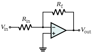
Zeroed impedance uses an inverting (usually op-amp) amplifier with enormously high gain . The output voltage is almost equal to the voltage drop across the impedance and completely neutralizes it. The circuit behaves as a short connection and a virtual ground appears at the input; so, it should not be driven by a constant voltage source. For this purpose, some circuits are driven by a constant current source or by a real voltage source with internal impedance: current-to-voltage converter (transimpedance amplifier), capacitive integrator (named also current integrator or charge amplifier), resistance-to-voltage converter (a resistive sensor connected in the place of the impedance ).

The rest of them have additional impedance connected in series to the input: voltage-to-current converter (transconductance amplifier), inverting amplifier, summing amplifier, inductive integrator, capacitive differentiator, resistive-capacitive integrator, capacitive-resistive differentiator, inductive-resistive differentiator, etc. The inverting integrators from this list are examples of useful and desired applications of the Miller effect in its extreme manifestation.
In all these op-amp inverting circuits with parallel negative feedback, the input current is increased to its maximum. It is determined only by the input voltage and the input impedance according to Ohm's law; it does not depend on the impedance .
Negative impedance with voltage inversion is implemented by applying both negative and positive feedback to an op-amp amplifier with a differential input. The input voltage source has to have internal impedance or it has to be connected through another impedance element to the input. Under these conditions, the input voltage of the circuit changes its polarity as the output voltage exceeds the voltage drop across the impedance ( ).


A typical application is a negative impedance converter with voltage inversion (VNIC).[5] It is interesting that the circuit input voltage has the same polarity as the output voltage, although it is applied to the inverting op-amp input; the input source has an opposite polarity to both the circuit input and output voltages.
Generalization of Miller arrangement edit
The original Miller effect is implemented by capacitive impedance connected between the two nodes. Miller theorem generalizes Miller effect as it implies arbitrary impedance connected between the nodes. It is supposed also a constant coefficient ; then the expressions above are valid. But modifying properties of Miller theorem exist even when these requirements are violated and this arrangement can be generalized further by dynamizing the impedance and the coefficient.
Non-linear element. Besides impedance, Miller arrangement can modify the IV characteristic of an arbitrary element. The circuit of a diode log converter is an example of a non-linear virtually zeroed resistance where the logarithmic forward IV curve of a diode is transformed to a vertical straight line overlapping the axis.

Not constant coefficient. If the coefficient varies, some exotic virtual elements can be obtained. A gyrator circuit is an example of such a virtual element where the resistance is modified so that to mimic inductance, capacitance or inversed resistance.

Dual Miller theorem (for currents) edit
Definition edit
There is also a dual version of Miller theorem that is based on Kirchhoff's current law (Miller theorem for currents): if there is a branch in a circuit with impedance connecting a node, where two currents and converge to ground, we can replace this branch by two conducting the referred currents, with impedances respectively equal to and , where . The dual theorem may be proved by replacing the two-port network by its equivalent and by applying the source absorption theorem.[3]


Explanation edit
Dual Miller theorem actually expresses the fact that connecting a second current source producing proportional current in parallel with the main input source and the impedance element changes the current flowing through it, the voltage and accordingly, the circuit impedance seen from the side of the input source. Depending on the direction, acts as a supplemental current source helping or opposing the main current source to create voltage across the impedance. The combination of the actual element and the second current source may be thought as of a new virtual element with dynamically modified impedance.

Implementation edit
Dual Miller theorem is usually implemented by an arrangement consisting of two voltage sources supplying the grounded impedance through floating impedances (see Fig. 3). The combinations of the voltage sources and belonging impedances form the two current sources – the main and the auxiliary one. As in the case of the main Miller theorem, the second voltage is usually produced by a voltage amplifier. Depending on the kind of the amplifier (inverting, non-inverting or differential) and the gain, the circuit input impedance may be virtually increased, infinite, decreased, zero or negative.
Applications edit
As the main Miller theorem, besides helping circuit analysis process, the dual version is a powerful tool for designing and understanding circuits based on modifying impedance by additional current. Typical applications are some exotic circuits with negative impedance as load cancellers,[6] capacitance neutralizers,[7] Howland current source and its derivative Deboo integrator.[8] In the last example (see Fig. 1 there), the Howland current source consists of an input voltage source , a positive resistor , a load (the capacitor acting as impedance ) and a negative impedance converter INIC ( and the op-amp). The input voltage source and the resistor constitute an imperfect current source passing current through the load (see Fig. 3 in the source). The INIC acts as a second current source passing "helping" current through the load. As a result, the total current flowing through the load is constant and the circuit impedance seen by the input source is increased. As a comparison, in a load canceller[permanent dead link], the INIC passes all the required current through the load; the circuit impedance seen from the side of the input source (the load impedance) is almost infinite.


List of specific applications based on Miller theorems edit
Below is a list of circuit solutions, phenomena and techniques based on the two Miller theorems.
- Potentiometric null-balance meter
- Electromechanical data recorders with a potentiometric servo system
- Emitter (source, cathode) follower
- Transistor amplifier with emitter (source, cathode) degeneration
- Transistor bootstrapped biasing circuits
- Transistor integrator
- Common-emitter (common-source, common-cathode) amplifying stages with stray capacitances
- Op-amp follower
- Op-amp non-inverting amplifier
- Op-amp bootstrapped AC follower with high input impedance
- Bilateral current source
- Negative impedance converter with current inversion (INIC)
- Negative impedance load canceller
- Negative impedance input capacitance canceller
- Howland current source
- Deboo integrator
- Op-amp inverting ammeter
- Op-amp voltage-to-current converter (transconductance amplifier)
- Op-amp current-to-voltage converter (transimpedance amplifier)
- Op-amp resistance-to-current converter
- Op-amp resistance-to-voltage converter
- Op-amp inverting amplifier
- Op-amp inverting summer
- Op-amp inverting capacitive integrator (current integrator, charge amplifier)
- Op-amp inverting resistive-capacitive integrator
- Op-amp inverting capacitive differentiator
- Op-amp inverting capacitive-resistive differentiator
- Op-amp inverting inductive integrator
- Op-amp inverting inductive-resistive differentiator, etc.
- Op-amp diode log converter
- Op-amp diode anti-log converter
- Op-amp inverting diode limiter (precision diode)
- Negative impedance converter with voltage inversion (VNIC), etc.
- Bootstrapping
- Input guarding of high impedance op-amp circuits
- Input-capacitance neutralization
- Virtual ground
- Miller effect
- Frequency op-amp compensation
- Negative impedance
- Load cancelling
See also edit
References edit
- ^ "Miscellaneous network theorems". Netlecturer.com. Archived from the original on 2012-03-21. Retrieved 2013-02-03.
- ^ a b c "EEE 194RF: Miller's theorem" (PDF). Retrieved 2013-02-03.
- ^ a b "Miller's theorem". Paginas.fe.up.pt. Retrieved 2013-02-03.
- ^ Working with High Impedance Op Amps Archived 2010-09-23 at the Wayback Machine AN-241
- ^ "Nonlinear Circuit Analysis – An Introduction" (PDF). Retrieved 2013-02-03.
- ^ Negative-resistance load canceller helps drive heavy loads
- ^ D. H. Sheingold (1964-01-01), "Impedance and admittance transformations using operational amplifiers", The Lightning Empiricist, 12 (1), retrieved 2014-06-22
- ^ "Consider the "Deboo" Single-Supply Integrator". Maxim-ic.com. 2002-08-29. Retrieved 2013-02-03.
Further reading edit
- Fundamentals of Microelectronics by Behzad Razavi
- Microelectronic Circuits by Adel Sedra and Kenneth Smith
- Fundamentals of RF Circuit Design by Jeremy Everard
External links edit
- Miller's theorem revisited
- New Results Related to Miller’s Theorem
- A network theorem dual to Miller's theorem
- Generalized Miller theorem and its applications
- The Feedback Decomposition Theorem (FDT): The evolution of Miller's Theorem
- An Accurate Calculation of Miller Effect on the Frequency Response and on the Input and Output Impedances of Feedback Amplifiers (using FDT)