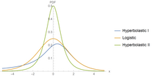
The hyperbolastic rate equation of type I, denoted H1, is given by

where ${\displaystyle x}$  is any real number and ${\displaystyle P\left(x\right)}$  is the population size at ${\displaystyle x}$ . The parameter ${\displaystyle M}$  represents carrying capacity, and parameters ${\displaystyle \delta }$  and ${\displaystyle \theta }$  jointly represent growth rate. The parameter ${\displaystyle \theta }$  gives the distance from a symmetric sigmoidal curve. Solving the hyperbolastic rate equation of type I for ${\displaystyle P\left(x\right)}$  gives

where ${\displaystyle \operatorname {arsinh} }$  is the inverse hyperbolic sine function. If one desires to use the initial condition ${\displaystyle P\left(x_{0}\right)=P_{0}}$ , then ${\displaystyle \alpha }$  can be expressed as

${\displaystyle \alpha ={\frac {M-P_{0}}{P_{0}}}e^{\delta x_{0}+\theta \operatorname {arsinh} (x_{0})}}$ .

If ${\displaystyle x_{0}=0}$ , then ${\displaystyle \alpha }$  reduces to

${\displaystyle \alpha ={\frac {M-P_{0}}{P_{0}}}}$ .

The hyperbolastic function of type I generalizes the logistic function. If the parameters ${\displaystyle \theta =0}$ , then it would become a logistic function. This function ${\displaystyle P(x)}$  is a hyperbolastic function of type I. The standard hyperbolastic function of type I is

${\displaystyle P(x)={\frac {1}{1+e^{-x-\theta \operatorname {arsinh} (x)}}}}$ .

The hyperbolastic rate equation of type II, denoted by H2, is defined as

${\displaystyle {\frac {dP(x)}{dx}}={\frac {\alpha \delta \gamma P^{2}(x)x^{\gamma -1}}{M}}\tanh \left({\frac {M-P(x)}{\alpha P(x)}}\right),}$ 

where ${\displaystyle \tanh }$  is the hyperbolic tangent function, ${\displaystyle M}$  is the carrying capacity, and both ${\displaystyle \delta }$  and ${\displaystyle \gamma >0}$  jointly determine the growth rate. In addition, the parameter ${\displaystyle \gamma }$  represents acceleration in the time course. Solving the hyperbolastic rate function of type II for ${\displaystyle P\left(x\right)}$  gives

${\displaystyle P(x)={\frac {M}{1+\alpha \operatorname {arsinh} \left(e^{-\delta x^{\gamma }}\right)}}}$ .

If one desires to use initial condition ${\displaystyle P(x_{0})=P_{0},}$  then ${\displaystyle \alpha }$  can be expressed as

${\displaystyle \alpha ={\frac {M-P_{0}}{P_{0}\operatorname {arsinh} \left(e^{-\delta x_{0}^{\gamma }}\right)}}}$ .

If ${\displaystyle x_{0}=0}$ , then ${\displaystyle \alpha }$  reduces to

${\displaystyle \alpha ={\frac {M-P_{0}}{P_{0}\operatorname {arsinh} (1)}}}$ .

The standard hyperbolastic function of type II is defined as

${\displaystyle P(x)={\frac {1}{1+\operatorname {arsinh} \left(e^{-x}\right)}}}$ .

The hyperbolastic rate equation of type III is denoted by H3 and has the form

${\displaystyle {\frac {dP(t)}{dt}}=\left(M-P\left(t\right)\right)\left(\delta \gamma t^{\gamma -1}+{\frac {\theta }{\sqrt {1+\theta ^{2}t^{2}}}}\right)}$ ,

where ${\displaystyle t}$  > 0. The parameter ${\displaystyle M}$  represents the carrying capacity, and the parameters ${\displaystyle \delta ,}$  ${\displaystyle \gamma ,}$  and ${\displaystyle \theta }$  jointly determine the growth rate. The parameter ${\displaystyle \gamma ,}$  represents acceleration of the time scale, while the size of ${\displaystyle \theta }$  represents distance from a symmetric sigmoidal curve. The solution to the differential equation of type III is

${\displaystyle P(t)=M-\alpha e^{-\delta t^{\gamma }-\operatorname {arsinh} (\theta t)}}$ ,

with the initial condition ${\displaystyle P\left(t_{0}\right)=P_{0}}$  we can express ${\displaystyle \alpha }$  as

${\displaystyle \alpha =\left(M-P_{0}\right)e^{\delta t_{0}^{\gamma }+\operatorname {arsinh} (\theta t_{0})}}$ .

The hyperbolastic distribution of type III is a three-parameter family of continuous probability distributions with scale parameters ${\displaystyle \delta }$  > 0, and ${\displaystyle \theta }$  ≥ 0 and parameter ${\displaystyle \gamma }$  as the shape parameter. When the parameter ${\displaystyle \theta }$  = 0, the hyperbolastic distribution of type III is reduced to the weibull distribution.^[11] The hyperbolastic cumulative distribution function of type III is given by

${\displaystyle F(x;\delta ,\gamma ,\theta )={\begin{cases}1-e^{-\delta x^{\gamma }-\operatorname {arsinh} (\theta x)}&x\geq 0,\\0&x<0\end{cases}}}$ ,

and its corresponding probability density function is

${\displaystyle f(x;\delta ,\gamma ,\theta )={\begin{cases}e^{-\delta x^{\gamma }-\operatorname {arsinh} (\theta x)}\left(\delta \gamma x^{\gamma -1}+{\frac {\theta }{\sqrt {1+\theta ^{2}x^{2}}}}\right)&x\geq 0,\\0&x<0\end{cases}}}$ .

The hazard function ${\displaystyle h}$  (or failure rate) is given by

${\displaystyle h\left(x;\delta ,\gamma ,\theta \right)=\delta \gamma x^{\gamma -1}+{\frac {\theta }{\sqrt {1+x^{2}\theta ^{2}}}}.}$ 

The survival function ${\displaystyle S}$  is given by

${\displaystyle S(x;\delta ,\gamma ,\theta )=e^{-\delta x^{\gamma }-\operatorname {arsinh} (\theta x)}.}$ 

The standard hyperbolastic cumulative distribution function of type III is defined as

${\displaystyle F\left(x\right)=1-e^{-x-\operatorname {arsinh} (x)}}$ ,

and its corresponding probability density function is

${\displaystyle f(x)=e^{-x-\operatorname {arsinh} (x)}\left(1+{\frac {1}{\sqrt {1+x^{2}}}}\right)}$ .

If one desires to calculate the point ${\displaystyle x}$  where the population reaches a percentage of its carrying capacity ${\displaystyle M}$ , then one can solve the equation

${\displaystyle P(x)=kM}$ 

for ${\displaystyle x}$ , where ${\displaystyle 0<k<1}$ . For instance, the half point can be found by setting ${\displaystyle k={\frac {1}{2}}}$ .

According to stem cell researchers at McGowan Institute for Regenerative Medicine at the University of Pittsburgh, "a newer model [called the hyperbolastic type III or] H3 is a differential equation that also describes the cell growth. This model allows for much more variation and has been proven to better predict growth."^[12]

The hyperbolastic growth models H1, H2, and H3 have been applied to analyze the growth of solid Ehrlich carcinoma using a variety of treatments.^[13]

In animal science,^[14] the hyperbolastic functions have been used for modeling broiler chicken growth.^[15][16] The hyperbolastic model of type III was used to determine the size of the recovering wound.^[17]

In the area of wound healing, the hyperbolastic models accurately representing the time course of healing. Such functions have been used to investigate variations in the healing velocity among different kinds of wounds and at different stages in the healing process taking into consideration the areas of trace elements, growth factors, diabetic wounds, and nutrition.^[18][19]

Another application of hyperbolastic functions is in the area of the stochastic diffusion process,^[20] whose mean function is a hyperbolastic curve. The main characteristics of the process are studied and the maximum likelihood estimation for the parameters of the process is considered.^[21] To this end, the firefly metaheuristic optimization algorithm is applied after bounding the parametric space by a stage wise procedure. Some examples based on simulated sample paths and real data illustrate this development. A sample path of a diffusion process models the trajectory of a particle embedded in a flowing fluid and subjected to random displacements due to collisions with other particles, which is called Brownian motion.^{[22][23][24][25][26]} The hyperbolastic function of type III was used to model the proliferation of both adult mesenchymal and embryonic stem cells;^{[27][28][29][30]} and, the hyperbolastic mixed model of type II has been used in modeling cervical cancer data.^[31] Hyperbolastic curves can be an important tool in analyzing cellular growth, the fitting of biological curves, the growth of phytoplankton, and instantaneous maturity rate.^{[32][33][34][35]}

In forest ecology and management, the hyperbolastic models have been applied to model the relationship between DBH and height.^[36]

The multivariable hyperbolastic model type III has been used to analyze the growth dynamics of phytoplankton taking into consideration the concentration of nutrients.^[37]

Hyperbolastic regressions are statistical models that utilize standard hyperbolastic functions to model a dichotomous or multinomial outcome variable. The purpose of hyperbolastic regression is to predict an outcome using a set of explanatory (independent) variables. These types of regressions are routinely used in many areas including medical, public health, dental, biomedical, as well as social, behavioral, and engineering sciences. For instance, binary regression analysis has been used to predict endoscopic lesions in iron deficiency anemia.^[38] In addition, binary regression was applied to differentiate between malignant and benign adnexal mass prior to surgery.^[39]

The binary hyperbolastic regression of type I edit

Let ${\displaystyle Y}$  be a binary outcome variable which can assume one of two mutually exclusive values, success or failure. If we code success as ${\displaystyle Y=1}$  and failure as ${\displaystyle Y=0}$ , then for parameter ${\displaystyle \theta \geq -1}$ , the hyperbolastic success probability of type I with a sample of size ${\displaystyle n}$  as a function of parameter ${\displaystyle \theta }$  and parameter vector ${\displaystyle {\boldsymbol {\beta }}=(\beta _{0},\beta _{1},\ldots ,\beta _{p})}$  given a ${\displaystyle p}$ -dimensional vector of explanatory variables is defined as ${\displaystyle \mathbf {x} _{i}=(x_{i1},\ x_{i2},\ldots ,\ x_{ip})^{T}}$ , where ${\displaystyle i=1,2,\ldots ,n}$ , is given by

${\displaystyle \pi (\mathbf {x} _{i};{\boldsymbol {\beta }})=P(y_{i}=1|\mathbf {x} _{i};{\boldsymbol {\beta }})={\frac {1}{1+e^{-(\beta _{0}+\sum _{s=1}^{p}{\beta _{s}x_{is}})-\theta \operatorname {arsinh} (\beta _{0}+\sum _{s=1}^{p}{\beta _{s}x_{is}})}}}}$ .

The odds of success is the ratio of the probability of success to the probability of failure. For binary hyperbolastic regression of type I, the odds of success is denoted by ${\displaystyle Odds_{H1}}$  and expressed by the equation

${\displaystyle Odds_{H1}=e^{\beta _{0}+\sum _{s=1}^{p}{\beta _{s}x_{is}}+\theta \operatorname {arsinh} (\beta _{0}+\sum _{s=1}^{p}{\beta _{s}x_{is}})}}$ .

The logarithm of ${\displaystyle Odds_{H1}}$  is called the logit of binary hyperbolastic regression of type I. The logit transformation is denoted by ${\displaystyle L_{H1}}$  and can be written as

${\displaystyle L_{H1}=\beta _{0}+\sum _{s=1}^{p}{\beta _{s}x_{is}}+\theta \operatorname {arsinh} [\beta _{0}+\sum _{s=1}^{p}{\beta _{s}x_{is}}]}$ .

Shannon information for binary hyperbolastic of type I (H1) edit

The Shannon information for the random variable ${\displaystyle Y}$  is defined as

${\displaystyle I(y)=-{log}_{b}P(y)}$ 

where the base of logarithm ${\displaystyle b>0}$  and ${\displaystyle b\neq 1}$ . For binary outcome, ${\displaystyle b}$  is equal to ${\displaystyle 2}$ .

For the binary hyperbolastic regression of type I, the information ${\displaystyle I(y)}$  is given by

${\displaystyle I(y)={\begin{cases}-log_{b}{\frac {1}{1+e^{-Z-\theta \operatorname {arsinh} (Z)}}}&y=1,\\-log_{b}{\frac {e^{-Z-\theta \operatorname {arsinh} (Z)}}{1+e^{-Z-\theta \operatorname {arsinh} (Z)}}}&y=0\end{cases}}}$ ,

where ${\displaystyle Z=\beta _{0}+\sum _{s=1}^{p}\beta _{s}x_{s}}$ , and ${\displaystyle x_{s}}$  is the ${\displaystyle s^{th}}$  input data. For a random sample of binary outcomes of size ${\displaystyle n}$ , the average empirical information for hyperbolastic H1 can be estimated by

${\displaystyle {\overline {I(y)}}={\begin{cases}-{\frac {1}{n}}\sum _{i=1}^{n}{log_{b}{\frac {1}{1+e^{-Z_{i}-\theta \operatorname {arsinh} (Z_{i})}}}}&y=1,\\-{\frac {1}{n}}\sum _{i=1}^{n}{log_{b}{\frac {e^{-Z_{i}-\theta \operatorname {arsinh} (Z_{i})}}{1+e^{-Z_{i}-\theta \operatorname {arsinh} (Z_{i})}}}}&y=0\end{cases}}}$ ,

where ${\displaystyle Z_{i}=\beta _{0}+\sum _{s=1}^{p}\beta _{s}x_{is}}$ , and ${\displaystyle x_{is}}$  is the ${\displaystyle s^{th}}$  input data for the ${\displaystyle i^{th}}$  observation.

Information Entropy for hyperbolastic H1 edit

Information entropy measures the loss of information in a transmitted message or signal. In machine learning applications, it is the number of bits necessary to transmit a randomly selected event from a probability distribution. For a discrete random variable ${\displaystyle Y}$ , the information entropy ${\displaystyle H}$  is defined as

${\displaystyle H=-\sum _{y\in Y}{P(y)\ {log}_{b}P(y)}}$ 

where ${\displaystyle P(y)}$  is the probability mass function for the random variable ${\displaystyle Y}$ .

The information entropy is the mathematical expectation of ${\displaystyle I(y)}$  with respect to probability mass function ${\displaystyle P(y)}$ . The Information entropy has many applications in machine learning and artificial intelligence such as classification modeling and decision trees. For the hyperbolastic H1, the entropy ${\displaystyle H}$  is equal to

${\displaystyle {\begin{aligned}H&=-\sum _{y\in \{0,1\}}{P(Y=y;\mathbf {x} ,{\boldsymbol {\beta }})log_{b}(P(Y=y;\mathbf {x} ,{\boldsymbol {\beta }}))}\\&=-[\pi (\mathbf {x} ;{\boldsymbol {\beta }})\ log_{b}(\pi (\mathbf {x} ;{\boldsymbol {\beta }})+(1-\pi (\mathbf {x} ;{\boldsymbol {\beta }}))log_{b}(1-\pi (\mathbf {x} ;{\boldsymbol {\beta }}))]\\&={log}_{b}(1+e^{-Z-\theta \operatorname {arsinh} (Z)})-{\frac {e^{-Z-\theta \operatorname {arsinh} (Z)}{log}_{b}(e^{-Z-\theta \operatorname {arsinh} (Z)})}{1+e^{-Z-\theta \operatorname {arsinh} (Z)}}}\end{aligned}}}$ 

The estimated average entropy for hyperbolastic H1 is denoted by ${\displaystyle {\bar {H}}}$  and is given by

${\displaystyle {\bar {H}}={\frac {1}{n}}\sum _{i=1}^{n}{[log_{b}(1+e^{{-Z}_{i}-\theta \operatorname {arsinh} (Z_{i})})-}{\frac {e^{{-Z}_{i}-\theta \operatorname {arsinh} (Z_{i})}\ {log}_{b}(e^{{-Z}_{i}-\theta \operatorname {arsinh} ((Z_{i})})}{1+e^{{-Z}_{i}-\theta \operatorname {arsinh} (Z_{i})}}}]}$ 

Binary Cross-entropy for hyperbolastic H1 edit

The binary cross-entropy compares the observed ${\displaystyle y\in \{0,1\}}$  with the predicted probabilities. The average binary cross-entropy for hyperbolastic H1 is denoted by ${\displaystyle {\overline {C}}}$  and is equal to

${\displaystyle {\begin{aligned}{\overline {C}}&=-{\frac {1}{n}}\sum _{i=1}^{n}{{[y}_{i}log_{b}(\pi (x_{i};{\boldsymbol {\beta }}))+}{(1-y}_{i})log_{b}(1-\pi (x_{i};{\boldsymbol {\beta }}))]\\&={\frac {1}{n}}\sum _{i=1}^{n}{[log_{b}(1+e^{{-Z}_{i}-\theta \operatorname {arsinh} (Z_{i})})-}{(1-y}_{i})log_{b}(e^{{-Z}_{i}-\theta \operatorname {arsinh} (Z_{i})})]\end{aligned}}}$ 

The binary hyperbolastic regression of type II edit

The hyperbolastic regression of type II is an alternative method for the analysis of binary data with robust properties. For the binary outcome variable ${\displaystyle Y}$ , the hyperbolastic success probability of type II is a function of a ${\displaystyle p}$ -dimensional vector of explanatory variables ${\displaystyle \mathbf {x} _{i}}$  given by

${\displaystyle \pi (\mathbf {x} _{i};{\boldsymbol {\beta }})=P(y_{i}=1|\mathbf {x} _{i};{\boldsymbol {\beta }})={\frac {1}{1+\operatorname {arsinh} [e^{-(\beta _{0}+\sum _{s=1}^{p}{\beta _{s}x_{is}})}]}}}$  ,

For the binary hyperbolastic regression of type II, the odds of success is denoted by ${\displaystyle Odds_{H2}}$  and is defined as

${\displaystyle Odds_{H2}={\frac {1}{\operatorname {arsinh} [e^{-(\beta _{0}+\sum _{s=1}^{p}{\beta _{s}x_{is}})}]}}.}$ 

The logit transformation ${\displaystyle L_{H2}}$  is given by

${\displaystyle L_{H2}=-\log {(\operatorname {arsinh} [e^{-(\beta _{0}+\sum _{s=1}^{p}{\beta _{s}x_{is}})}])}}$ 

Shannon information for binary hyperbolastic of type II (H2) edit

For the binary hyperbolastic regression H2, the Shannon information ${\displaystyle I(y)}$  is given by

${\displaystyle I(y)={\begin{cases}-log_{b}{\frac {1}{1+arsinh(e^{-Z})}}&y=1\\-log_{b}{\frac {arsinh(e^{-Z})}{1+arsinh(e^{-Z})}}&y=0\end{cases}}}$ 

where ${\displaystyle Z=\beta _{0}+\sum _{s=1}^{p}\beta _{s}x_{s}}$ , and ${\displaystyle x_{s}}$  is the ${\displaystyle s^{th}}$  input data. For a random sample of binary outcomes of size ${\displaystyle n}$ , the average empirical information for hyperbolastic H2 is estimated by

${\displaystyle {\overline {I(y)}}={\begin{cases}-{\frac {1}{n}}\sum _{i=1}^{n}log_{b}{\frac {1}{1+arsinh(e^{-Z_{i}})}}&y=1\\-{\frac {1}{n}}\sum _{i=1}^{n}log_{b}{\frac {arsinh(e^{-Z_{i}})}{1+arsinh(e^{-Z_{i}})}}&y=0\end{cases}}}$ 

where ${\displaystyle Z_{i}=\beta _{0}+\sum _{s=1}^{p}\beta _{s}x_{is}}$ , and ${\displaystyle x_{is}}$  is the ${\displaystyle s^{th}}$  input data for the ${\displaystyle i^{th}}$  observation.

Information Entropy for hyperbolastic H2 edit

For the hyperbolastic H2, the information entropy ${\displaystyle H}$  is equal to

${\displaystyle {\begin{aligned}H&=-\sum _{y\in \{0,1\}}{P(Y=y;\mathbf {x} ,{\boldsymbol {\beta }})log_{b}(P(Y=y;\mathbf {x} ,{\boldsymbol {\beta }}))}\\&=-[\pi (\mathbf {x} ;{\boldsymbol {\beta }})\ log_{b}(\pi (\mathbf {x} ;{\boldsymbol {\beta }}))+(1-\pi (\mathbf {x} ;{\boldsymbol {\beta }}))log_{b}(1-\pi (\mathbf {x} ;{\boldsymbol {\beta }}))]\\&=log_{b}(1+arsinh(e^{-Z}))-{\frac {arsinh(e^{-Z})log_{b}(arsinh(e^{-Z}))}{1+arsinh(e^{-Z})}}\end{aligned}}}$ 

and the estimated average entropy ${\displaystyle {\bar {H}}}$  for hyperbolastic H2 is

${\displaystyle {\bar {H}}={\frac {1}{n}}\sum _{i=1}^{n}{[log_{b}(1+{arsinh(e}^{{-Z}_{i}}))-}{\frac {{arsinh(e}^{{-Z}_{i}})\ {log}_{b}{(arsinh(e}^{{-Z}_{i}}))}{1+{arsinh(e}^{{-Z}_{i}})}}]}$ 

Binary Cross-entropy for hyperbolastic H2 edit

The average binary cross-entropy ${\displaystyle {\overline {C}}}$  for hyperbolastic H2 is

${\displaystyle {\begin{aligned}{\overline {C}}&=-{\frac {1}{n}}\sum _{i=1}^{n}{{[y}_{i}log_{b}(\pi (x_{i};\beta ))+}{(1-y}_{i})log_{b}(1-\pi (x_{i};\beta ))]\\&={\frac {1}{n}}\sum _{i=1}^{n}{[log_{b}(1+{arsinh(e}^{{-Z}_{i}}))-}{(1-y}_{i})log_{b}({arsinh(e}^{{-Z}_{i}}))]\end{aligned}}}$ 

Parameter estimation for the binary hyperbolastic regression of type I and II edit

The estimate of the parameter vector ${\displaystyle {\boldsymbol {\beta }}}$  can be obtained by maximizing the log-likelihood function

${\displaystyle {\hat {\beta }}={\underset {\boldsymbol {\beta }}{\operatorname {argmax} }}{\sum _{i=1}^{n}[y_{i}ln(\pi (\mathbf {x} _{i};{\boldsymbol {\beta }}))+(1-y_{i})ln(1-\pi (\mathbf {x} _{i};{\boldsymbol {\beta }}))]}}$ 

where ${\displaystyle \pi (\mathbf {x} _{i};{\boldsymbol {\beta }})}$  is defined according to one of the two types of hyberbolastic functions used.

The multinomial hyperbolastic regression of type I and II edit

The generalization of the binary hyperbolastic regression to multinomial hyperbolastic regression has a response variable ${\displaystyle y_{i}}$  for individual ${\displaystyle i}$  with ${\displaystyle k}$  categories (i.e. ${\displaystyle y_{i}\in \{1,2,\ldots ,k\}}$ ). When ${\displaystyle k=2}$ , this model reduces to a binary hyperbolastic regression. For each ${\displaystyle i=1,2,\ldots ,n}$ , we form ${\displaystyle k}$  indicator variables ${\displaystyle y_{ij}}$  where

${\displaystyle y_{ij}={\begin{cases}1&{\text{if }}y_{i}=j,\\0&{\text{if }}y_{i}\neq j\end{cases}}}$ ,

meaning that ${\displaystyle y_{ij}=1}$  whenever the ${\displaystyle i^{th}}$  response is in category ${\displaystyle j}$  and ${\displaystyle 0}$  otherwise.

Define parameter vector ${\displaystyle {\boldsymbol {\beta }}_{j}=(\beta _{j0},\beta _{j1},\ldots ,\beta _{jp})}$  in a ${\displaystyle p+1}$ -dimensional Euclidean space and ${\displaystyle {\boldsymbol {\beta }}=({\boldsymbol {\beta }}_{1},\ldots ,{\boldsymbol {\beta }}_{k-1})^{T}}$ .

Using category 1 as a reference and ${\displaystyle \pi _{1}(\mathbf {x} _{i};{\boldsymbol {\beta }})}$  as its corresponding probability function, the multinomial hyperbolastic regression of type I probabilities are defined as

${\displaystyle \pi _{1}(\mathbf {x} _{i};{\boldsymbol {\beta }})=P(y_{i}=1|\mathbf {x} _{i};{\boldsymbol {\beta }})={\frac {1}{1+\sum _{s=2}^{k}e^{-\eta _{s}(\mathbf {x} _{i};{\boldsymbol {\beta }})-\theta \operatorname {arsinh} [\eta _{s}(\mathbf {x} _{i};{\boldsymbol {\beta }})]}}}}$ 

and for ${\displaystyle j=2,\ldots ,k}$ ,

${\displaystyle \pi _{j}(\mathbf {x} _{i};{\boldsymbol {\beta }})=P(y_{i}=j|\mathbf {x} _{i};{\boldsymbol {\beta }})={\frac {e^{-\eta _{j}(\mathbf {x} _{i};{\boldsymbol {\beta }})-\theta \operatorname {arsinh} [\eta _{j}(\mathbf {x} _{i};{\boldsymbol {\beta }})]}}{1+\sum _{s=2}^{k}e^{-\eta _{s}(\mathbf {x} _{i};{\boldsymbol {\beta }})-\theta \operatorname {arsinh} [\eta _{s}(\mathbf {x} _{i};{\boldsymbol {\beta }})]}}}}$ 

Similarly, for the multinomial hyperbolastic regression of type II we have

${\displaystyle \pi _{1}(\mathbf {x} _{i};{\boldsymbol {\beta }})=P(y_{i}=1|\mathbf {x} _{i};{\boldsymbol {\beta }})={\frac {1}{1+\sum _{s=2}^{k}arsinh[e^{-\eta _{s}(\mathbf {x} _{i};{\boldsymbol {\beta }})}]}}}$ 

and for ${\displaystyle j=2,\ldots ,k}$ ,

${\displaystyle \pi _{j}(\mathbf {x} _{i};{\boldsymbol {\beta }})=P(y_{i}=j|\mathbf {x} _{i};{\boldsymbol {\beta }})={\frac {arsinh[e^{-\eta _{j}(\mathbf {x} _{i};{\boldsymbol {\beta }})}]}{1+\sum _{s=2}^{k}arsinh[e^{-\eta _{s}(\mathbf {x} _{i};{\boldsymbol {\beta }})}]}}}$ 

where ${\displaystyle \eta _{s}(\mathbf {x} _{i};{\boldsymbol {\beta }})=\beta _{s0}+\sum _{l=1}^{p}\beta _{sl}x_{il}}$  with ${\displaystyle s=2,\dots ,k}$  and ${\displaystyle i=1,\dots ,n}$ .

The choice of ${\displaystyle \pi _{i}(\mathbf {x_{i}} ;{\boldsymbol {\beta }})}$  is dependent on the choice of hyperbolastic H1 or H2.

Shannon Information for multiclass hyperbolastic H1 or H2 edit

For the multiclass ${\displaystyle (j=1,2,\dots ,k)}$ , the Shannon information ${\displaystyle I_{j}}$  is

${\displaystyle I_{j}=-log_{b}(\pi _{j}(\mathbf {x} ;{\boldsymbol {\beta }}))}$ .

For a random sample of size ${\displaystyle n}$ , the empirical multiclass information can be estimated by

${\displaystyle {\overline {I_{j}}}=-{\frac {1}{n}}\sum _{i=1}^{n}{log_{b}(\pi _{j}(\mathbf {x_{i}} ;{\boldsymbol {\beta }}))}}$ .

Multiclass Entropy in Information Theory edit

For a discrete random variable ${\displaystyle Y}$ , the multiclass information entropy is defined as

${\displaystyle H=-\sum _{y\in Y}{P(y)\ {log}_{b}P(y)}}$ 

where ${\displaystyle P(y)}$  is the probability mass function for the multiclass random variable ${\displaystyle Y}$ .

For the hyperbolastic H1 or H2, the multiclass entropy ${\displaystyle H}$  is equal to

${\displaystyle H=-\sum _{j=1}^{k}{[\pi _{j}(\mathbf {x} ;{\boldsymbol {\beta }})log_{b}(\pi _{j}(\mathbf {x} ;{\boldsymbol {\beta }}))]}}$ 

The estimated average multiclass entropy ${\displaystyle {\overline {H}}}$  is equal to

${\displaystyle {\overline {H}}=-{\frac {1}{n}}\sum _{i=1}^{n}{\sum _{j=1}^{k}{[\pi _{j}(\mathbf {x_{i}} ;{\boldsymbol {\beta }})log_{b}(\pi _{j}(\mathbf {x_{i}} ;{\boldsymbol {\beta }}))]}}}$ 

Multiclass Cross-entropy for hyperbolastic H1 or H2 edit

Multiclass cross-entropy compares the observed multiclass output with the predicted probabilities. For a random sample of multiclass outcomes of size ${\displaystyle n}$ , the average multiclass cross-entropy ${\displaystyle {\overline {C}}}$  for hyperbolastic H1 or H2 can be estimated by

${\displaystyle {\overline {C}}=-{\frac {1}{n}}\sum _{i=1}^{n}{\sum _{j=1}^{k}{[y_{ij}log_{b}(\pi _{j}(\mathbf {x_{i}} ;{\boldsymbol {\beta }}))]}}}$ 

The log-odds of membership in category ${\displaystyle j}$  versus the reference category 1, denoted by ${\displaystyle o_{j}(\mathbf {x} _{i};{\boldsymbol {\beta }})}$ , is equal to

${\displaystyle o_{j}(\mathbf {x} _{i};{\boldsymbol {\beta }})=ln[{\frac {\pi _{j}(\mathbf {x} _{i};{\boldsymbol {\beta }})}{\pi _{1}(\mathbf {x} _{i};{\boldsymbol {\beta }})}}]}$ 

where ${\displaystyle j=2,\ldots ,k}$  and ${\displaystyle i=1,\ldots ,n}$ . The estimated parameter matrix ${\displaystyle {\hat {\boldsymbol {\beta }}}}$  of multinomial hyperbolastic regression is obtained by maximizing the log-likelihood function. The maximum likelihood estimates of the parameter matrix ${\displaystyle {\boldsymbol {\beta }}}$  is

${\displaystyle {\boldsymbol {\hat {\beta }}}={\underset {\boldsymbol {\beta }}{\operatorname {argmax} }}{\sum _{i=1}^{n}(y_{i1}ln[\pi _{1}(\mathbf {x} _{i};{\boldsymbol {\beta }})]+y_{i2}ln[\pi _{2}(\mathbf {x} _{i};{\boldsymbol {\beta }})]+\ldots +y_{ik}ln[\pi _{k}(\mathbf {x} _{i};{\boldsymbol {\beta }})])}}$