


Summary
In mathematics, physics, and engineering, a Euclidean vector or simply a vector (sometimes called a geometric vector[1] or spatial vector[2]) is a geometric object that has magnitude (or length) and direction. Euclidean vectors can be added and scaled to form a vector space. A Euclidean vector is frequently represented by a directed line segment, or graphically as an arrow connecting an initial point A with a terminal point B,[3] and denoted by


A vector is what is needed to "carry" the point A to the point B; the Latin word vector means "carrier".[4] It was first used by 18th century astronomers investigating planetary revolution around the Sun.[5] The magnitude of the vector is the distance between the two points, and the direction refers to the direction of displacement from A to B. Many algebraic operations on real numbers such as addition, subtraction, multiplication, and negation have close analogues for vectors,[6] operations which obey the familiar algebraic laws of commutativity, associativity, and distributivity. These operations and associated laws qualify Euclidean vectors as an example of the more generalized concept of vectors defined simply as elements of a vector space.
Vectors play an important role in physics: the velocity and acceleration of a moving object and the forces acting on it can all be described with vectors.[7] Many other physical quantities can be usefully thought of as vectors. Although most of them do not represent distances (except, for example, position or displacement), their magnitude and direction can still be represented by the length and direction of an arrow. The mathematical representation of a physical vector depends on the coordinate system used to describe it. Other vector-like objects that describe physical quantities and transform in a similar way under changes of the coordinate system include pseudovectors and tensors.[8]
History edit
The vector concept, as it is known today, is the result of a gradual development over a period of more than 200 years. About a dozen people contributed significantly to its development.[9] In 1835, Giusto Bellavitis abstracted the basic idea when he established the concept of equipollence. Working in a Euclidean plane, he made equipollent any pair of parallel line segments of the same length and orientation. Essentially, he realized an equivalence relation on the pairs of points (bipoints) in the plane, and thus erected the first space of vectors in the plane.[9]: 52–4 The term vector was introduced by William Rowan Hamilton as part of a quaternion, which is a sum q = s + v of a real number s (also called scalar) and a 3-dimensional vector. Like Bellavitis, Hamilton viewed vectors as representative of classes of equipollent directed segments. As complex numbers use an imaginary unit to complement the real line, Hamilton considered the vector v to be the imaginary part of a quaternion:[10]
The algebraically imaginary part, being geometrically constructed by a straight line, or radius vector, which has, in general, for each determined quaternion, a determined length and determined direction in space, may be called the vector part, or simply the vector of the quaternion.
Several other mathematicians developed vector-like systems in the middle of the nineteenth century, including Augustin Cauchy, Hermann Grassmann, August Möbius, Comte de Saint-Venant, and Matthew O'Brien. Grassmann's 1840 work Theorie der Ebbe und Flut (Theory of the Ebb and Flow) was the first system of spatial analysis that is similar to today's system, and had ideas corresponding to the cross product, scalar product and vector differentiation. Grassmann's work was largely neglected until the 1870s.[9] Peter Guthrie Tait carried the quaternion standard after Hamilton. His 1867 Elementary Treatise of Quaternions included extensive treatment of the nabla or del operator ∇. In 1878, Elements of Dynamic was published by William Kingdon Clifford. Clifford simplified the quaternion study by isolating the dot product and cross product of two vectors from the complete quaternion product. This approach made vector calculations available to engineers—and others working in three dimensions and skeptical of the fourth.
Josiah Willard Gibbs, who was exposed to quaternions through James Clerk Maxwell's Treatise on Electricity and Magnetism, separated off their vector part for independent treatment. The first half of Gibbs's Elements of Vector Analysis, published in 1881, presents what is essentially the modern system of vector analysis.[9][6] In 1901, Edwin Bidwell Wilson published Vector Analysis, adapted from Gibbs's lectures, which banished any mention of quaternions in the development of vector calculus.
Overview edit
In physics and engineering, a vector is typically regarded as a geometric entity characterized by a magnitude and a direction. It is formally defined as a directed line segment, or arrow, in a Euclidean space.[11] In pure mathematics, a vector is defined more generally as any element of a vector space. In this context, vectors are abstract entities which may or may not be characterized by a magnitude and a direction. This generalized definition implies that the above-mentioned geometric entities are a special kind of vectors, as they are elements of a special kind of vector space called Euclidean space. This particular article is about vectors strictly defined as arrows in Euclidean space. When it becomes necessary to distinguish these special vectors from vectors as defined in pure mathematics, they are sometimes referred to as geometric, spatial, or Euclidean vectors.
Being an arrow, a Euclidean vector possesses a definite initial point and terminal point. A vector with fixed initial and terminal point is called a bound vector.[12] When only the magnitude and direction of the vector matter, then the particular initial point is of no importance, and the vector is called a free vector. Thus two arrows and in space represent the same free vector if they have the same magnitude and direction: that is, they are equipollent if the quadrilateral ABB′A′ is a parallelogram. If the Euclidean space is equipped with a choice of origin, then a free vector is equivalent to the bound vector of the same magnitude and direction whose initial point is the origin. The term vector also has generalizations to higher dimensions, and to more formal approaches with much wider applications.


Further information edit
In classical Euclidean geometry (i.e., synthetic geometry), vectors were introduced (during the 19th century) as equivalence classes under equipollence, of ordered pairs of points; two pairs (A, B) and (C, D) being equipollent if the points A, B, D, C, in this order, form a parallelogram. Such an equivalence class is called a vector, more precisely, a Euclidean vector.[13] The equivalence class of (A, B) is often denoted

A Euclidean vector is thus an equivalence class of directed segments with the same magnitude (e.g., the length of the line segment (A, B)) and same direction (e.g., the direction from A to B).[14] In physics, Euclidean vectors are used to represent physical quantities that have both magnitude and direction, but are not located at a specific place, in contrast to scalars, which have no direction.[7] For example, velocity, forces and acceleration are represented by vectors.
In modern geometry, Euclidean spaces are often defined from linear algebra. More precisely, a Euclidean space E is defined as a set to which is associated an inner product space of finite dimension over the reals and a group action of the additive group of which is free and transitive (See Affine space for details of this construction). The elements of are called translations. It has been proven that the two definitions of Euclidean spaces are equivalent, and that the equivalence classes under equipollence may be identified with translations.


Sometimes, Euclidean vectors are considered without reference to a Euclidean space. In this case, a Euclidean vector is an element of a normed vector space of finite dimension over the reals, or, typically, an element of equipped with the dot product. This makes sense, as the addition in such a vector space acts freely and transitively on the vector space itself. That is, is a Euclidean space, with itself as an associated vector space, and the dot product as an inner product.

The Euclidean space is often presented as the Euclidean space of dimension n. This is motivated by the fact that every Euclidean space of dimension n is isomorphic to the Euclidean space More precisely, given such a Euclidean space, one may choose any point O as an origin. By Gram–Schmidt process, one may also find an orthonormal basis of the associated vector space (a basis such that the inner product of two basis vectors is 0 if they are different and 1 if they are equal). This defines Cartesian coordinates of any point P of the space, as the coordinates on this basis of the vector These choices define an isomorphism of the given Euclidean space onto by mapping any point to the n-tuple of its Cartesian coordinates, and every vector to its coordinate vector.


Examples in one dimension edit
Since the physicist's concept of force has a direction and a magnitude, it may be seen as a vector. As an example, consider a rightward force F of 15 newtons. If the positive axis is also directed rightward, then F is represented by the vector 15 N, and if positive points leftward, then the vector for F is −15 N. In either case, the magnitude of the vector is 15 N. Likewise, the vector representation of a displacement Δs of 4 meters would be 4 m or −4 m, depending on its direction, and its magnitude would be 4 m regardless.
In physics and engineering edit
Vectors are fundamental in the physical sciences. They can be used to represent any quantity that has magnitude, has direction, and which adheres to the rules of vector addition. An example is velocity, the magnitude of which is speed. For instance, the velocity 5 meters per second upward could be represented by the vector (0, 5) (in 2 dimensions with the positive y-axis as 'up'). Another quantity represented by a vector is force, since it has a magnitude and direction and follows the rules of vector addition.[7] Vectors also describe many other physical quantities, such as linear displacement, displacement, linear acceleration, angular acceleration, linear momentum, and angular momentum. Other physical vectors, such as the electric and magnetic field, are represented as a system of vectors at each point of a physical space; that is, a vector field. Examples of quantities that have magnitude and direction, but fail to follow the rules of vector addition, are angular displacement and electric current. Consequently, these are not vectors.
In Cartesian space edit
In the Cartesian coordinate system, a bound vector can be represented by identifying the coordinates of its initial and terminal point. For instance, the points A = (1, 0, 0) and B = (0, 1, 0) in space determine the bound vector pointing from the point x = 1 on the x-axis to the point y = 1 on the y-axis.

In Cartesian coordinates, a free vector may be thought of in terms of a corresponding bound vector, in this sense, whose initial point has the coordinates of the origin O = (0, 0, 0). It is then determined by the coordinates of that bound vector's terminal point. Thus the free vector represented by (1, 0, 0) is a vector of unit length—pointing along the direction of the positive x-axis.
This coordinate representation of free vectors allows their algebraic features to be expressed in a convenient numerical fashion. For example, the sum of the two (free) vectors (1, 2, 3) and (−2, 0, 4) is the (free) vector

Euclidean and affine vectors edit
In the geometrical and physical settings, it is sometimes possible to associate, in a natural way, a length or magnitude and a direction to vectors. In addition, the notion of direction is strictly associated with the notion of an angle between two vectors. If the dot product of two vectors is defined—a scalar-valued product of two vectors—then it is also possible to define a length; the dot product gives a convenient algebraic characterization of both angle (a function of the dot product between any two non-zero vectors) and length (the square root of the dot product of a vector by itself). In three dimensions, it is further possible to define the cross product, which supplies an algebraic characterization of the area and orientation in space of the parallelogram defined by two vectors (used as sides of the parallelogram). In any dimension (and, in particular, higher dimensions), it is possible to define the exterior product, which (among other things) supplies an algebraic characterization of the area and orientation in space of the n-dimensional parallelotope defined by n vectors.
In a pseudo-Euclidean space, a vector's squared length can be positive, negative, or zero. An important example is Minkowski space (which is important to our understanding of special relativity).
However, it is not always possible or desirable to define the length of a vector. This more general type of spatial vector is the subject of vector spaces (for free vectors) and affine spaces (for bound vectors, as each represented by an ordered pair of "points"). One physical example comes from thermodynamics, where many quantities of interest can be considered vectors in a space with no notion of length or angle.[15]
Generalizations edit
In physics, as well as mathematics, a vector is often identified with a tuple of components, or list of numbers, that act as scalar coefficients for a set of basis vectors. When the basis is transformed, for example by rotation or stretching, then the components of any vector in terms of that basis also transform in an opposite sense. The vector itself has not changed, but the basis has, so the components of the vector must change to compensate. The vector is called covariant or contravariant, depending on how the transformation of the vector's components is related to the transformation of the basis. In general, contravariant vectors are "regular vectors" with units of distance (such as a displacement), or distance times some other unit (such as velocity or acceleration); covariant vectors, on the other hand, have units of one-over-distance such as gradient. If you change units (a special case of a change of basis) from meters to millimeters, a scale factor of 1/1000, a displacement of 1 m becomes 1000 mm—a contravariant change in numerical value. In contrast, a gradient of 1 K/m becomes 0.001 K/mm—a covariant change in value (for more, see covariance and contravariance of vectors). Tensors are another type of quantity that behave in this way; a vector is one type of tensor.
In pure mathematics, a vector is any element of a vector space over some field and is often represented as a coordinate vector. The vectors described in this article are a very special case of this general definition, because they are contravariant with respect to the ambient space. Contravariance captures the physical intuition behind the idea that a vector has "magnitude and direction".
Representations edit

Vectors are usually denoted in lowercase boldface, as in , and , or in lowercase italic boldface, as in a. (Uppercase letters are typically used to represent matrices.) Other conventions include or a, especially in handwriting. Alternatively, some use a tilde (~) or a wavy underline drawn beneath the symbol, e.g. , which is a convention for indicating boldface type. If the vector represents a directed distance or displacement from a point A to a point B (see figure), it can also be denoted as or AB. In German literature, it was especially common to represent vectors with small fraktur letters such as .


Vectors are usually shown in graphs or other diagrams as arrows (directed line segments), as illustrated in the figure. Here, the point A is called the origin, tail, base, or initial point, and the point B is called the head, tip, endpoint, terminal point or final point. The length of the arrow is proportional to the vector's magnitude, while the direction in which the arrow points indicates the vector's direction.

On a two-dimensional diagram, a vector perpendicular to the plane of the diagram is sometimes desired. These vectors are commonly shown as small circles. A circle with a dot at its centre (Unicode U+2299 ⊙) indicates a vector pointing out of the front of the diagram, toward the viewer. A circle with a cross inscribed in it (Unicode U+2297 ⊗) indicates a vector pointing into and behind the diagram. These can be thought of as viewing the tip of an arrow head on and viewing the flights of an arrow from the back.
In order to calculate with vectors, the graphical representation may be too cumbersome. Vectors in an n-dimensional Euclidean space can be represented as coordinate vectors in a Cartesian coordinate system. The endpoint of a vector can be identified with an ordered list of n real numbers (n-tuple). These numbers are the coordinates of the endpoint of the vector, with respect to a given Cartesian coordinate system, and are typically called the scalar components (or scalar projections) of the vector on the axes of the coordinate system.
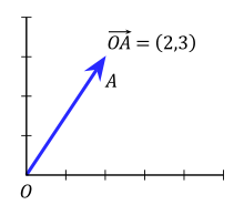
As an example in two dimensions (see figure), the vector from the origin O = (0, 0) to the point A = (2, 3) is simply written as

The notion that the tail of the vector coincides with the origin is implicit and easily understood. Thus, the more explicit notation is usually deemed not necessary (and is indeed rarely used).

In three dimensional Euclidean space (or R3), vectors are identified with triples of scalar components:


This can be generalised to n-dimensional Euclidean space (or Rn).

These numbers are often arranged into a column vector or row vector, particularly when dealing with matrices, as follows:
![{\displaystyle \mathbf {a} ={\begin{bmatrix}a_{1}\\a_{2}\\a_{3}\\\end{bmatrix}}=[a_{1}\ a_{2}\ a_{3}]^{\operatorname {T} }.}](https://wikimedia.org/api/rest_v1/media/math/render/svg/0a4d592431150c7ec8a51217d87dae2ed1224df2)
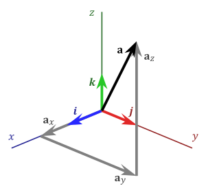
Another way to represent a vector in n-dimensions is to introduce the standard basis vectors. For instance, in three dimensions, there are three of them:


or

where a1, a2, a3 are called the vector components (or vector projections) of a on the basis vectors or, equivalently, on the corresponding Cartesian axes x, y, and z (see figure), while a1, a2, a3 are the respective scalar components (or scalar projections).
In introductory physics textbooks, the standard basis vectors are often denoted instead (or , in which the hat symbol typically denotes unit vectors). In this case, the scalar and vector components are denoted respectively ax, ay, az, and ax, ay, az (note the difference in boldface). Thus,


The notation ei is compatible with the index notation and the summation convention commonly used in higher level mathematics, physics, and engineering.
Decomposition or resolution edit
As explained above, a vector is often described by a set of vector components that add up to form the given vector. Typically, these components are the projections of the vector on a set of mutually perpendicular reference axes (basis vectors). The vector is said to be decomposed or resolved with respect to that set.

The decomposition or resolution[16] of a vector into components is not unique, because it depends on the choice of the axes on which the vector is projected.
Moreover, the use of Cartesian unit vectors such as as a basis in which to represent a vector is not mandated. Vectors can also be expressed in terms of an arbitrary basis, including the unit vectors of a cylindrical coordinate system ( ) or spherical coordinate system ( ). The latter two choices are more convenient for solving problems which possess cylindrical or spherical symmetry, respectively.


The choice of a basis does not affect the properties of a vector or its behaviour under transformations.
A vector can also be broken up with respect to "non-fixed" basis vectors that change their orientation as a function of time or space. For example, a vector in three-dimensional space can be decomposed with respect to two axes, respectively normal, and tangent to a surface (see figure). Moreover, the radial and tangential components of a vector relate to the radius of rotation of an object. The former is parallel to the radius and the latter is orthogonal to it.[17]
In these cases, each of the components may be in turn decomposed with respect to a fixed coordinate system or basis set (e.g., a global coordinate system, or inertial reference frame).
Basic properties edit
The following section uses the Cartesian coordinate system with basis vectors


Equality edit
Two vectors are said to be equal if they have the same magnitude and direction. Equivalently they will be equal if their coordinates are equal. So two vectors


Opposite, parallel, and antiparallel vectors edit
Two vectors are opposite if they have the same magnitude but opposite direction. So two vectors
and
are opposite if

Two vectors are parallel if they have the same direction but not necessarily the same magnitude, or antiparallel if they have opposite direction but not necessarily the same magnitude.[18]
Addition and subtraction edit
The sum of a and b of two vectors may be defined as

The addition may be represented graphically by placing the tail of the arrow b at the head of the arrow a, and then drawing an arrow from the tail of a to the head of b. The new arrow drawn represents the vector a + b, as illustrated below:[7]

This addition method is sometimes called the parallelogram rule because a and b form the sides of a parallelogram and a + b is one of the diagonals. If a and b are bound vectors that have the same base point, this point will also be the base point of a + b. One can check geometrically that a + b = b + a and (a + b) + c = a + (b + c).
The difference of a and b is

Subtraction of two vectors can be geometrically illustrated as follows: to subtract b from a, place the tails of a and b at the same point, and then draw an arrow from the head of b to the head of a. This new arrow represents the vector (-b) + a, with (-b) being the opposite of b, see drawing. And (-b) + a = a − b.

Scalar multiplication edit

A vector may also be multiplied, or re-scaled, by a real number r. In the context of conventional vector algebra, these real numbers are often called scalars (from scale) to distinguish them from vectors. The operation of multiplying a vector by a scalar is called scalar multiplication. The resulting vector is

Intuitively, multiplying by a scalar r stretches a vector out by a factor of r. Geometrically, this can be visualized (at least in the case when r is an integer) as placing r copies of the vector in a line where the endpoint of one vector is the initial point of the next vector.
If r is negative, then the vector changes direction: it flips around by an angle of 180°. Two examples (r = −1 and r = 2) are given below:

Scalar multiplication is distributive over vector addition in the following sense: r(a + b) = ra + rb for all vectors a and b and all scalars r. One can also show that a − b = a + (−1)b.
Length edit
The length or magnitude or norm of the vector a is denoted by ‖a‖ or, less commonly, |a|, which is not to be confused with the absolute value (a scalar "norm").
The length of the vector a can be computed with the Euclidean norm,

which is a consequence of the Pythagorean theorem since the basis vectors e1, e2, e3 are orthogonal unit vectors.
This happens to be equal to the square root of the dot product, discussed below, of the vector with itself:

Unit vector edit

A unit vector is any vector with a length of one; normally unit vectors are used simply to indicate direction. A vector of arbitrary length can be divided by its length to create a unit vector.[14] This is known as normalizing a vector. A unit vector is often indicated with a hat as in â.
To normalize a vector a = (a1, a2, a3), scale the vector by the reciprocal of its length ‖a‖. That is:

Zero vector edit
The zero vector is the vector with length zero. Written out in coordinates, the vector is (0, 0, 0), and it is commonly denoted , 0, or simply 0. Unlike any other vector, it has an arbitrary or indeterminate direction, and cannot be normalized (that is, there is no unit vector that is a multiple of the zero vector). The sum of the zero vector with any vector a is a (that is, 0 + a = a).

Dot product edit
The dot product of two vectors a and b (sometimes called the inner product, or, since its result is a scalar, the scalar product) is denoted by a ∙ b, and is defined as:

where θ is the measure of the angle between a and b (see trigonometric function for an explanation of cosine). Geometrically, this means that a and b are drawn with a common start point, and then the length of a is multiplied with the length of the component of b that points in the same direction as a.
The dot product can also be defined as the sum of the products of the components of each vector as

Cross product edit
The cross product (also called the vector product or outer product) is only meaningful in three or seven dimensions. The cross product differs from the dot product primarily in that the result of the cross product of two vectors is a vector. The cross product, denoted a × b, is a vector perpendicular to both a and b and is defined as

where θ is the measure of the angle between a and b, and n is a unit vector perpendicular to both a and b which completes a right-handed system. The right-handedness constraint is necessary because there exist two unit vectors that are perpendicular to both a and b, namely, n and (−n).
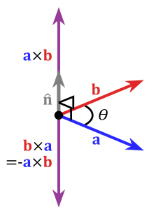
The cross product a × b is defined so that a, b, and a × b also becomes a right-handed system (although a and b are not necessarily orthogonal). This is the right-hand rule.
The length of a × b can be interpreted as the area of the parallelogram having a and b as sides.
The cross product can be written as

For arbitrary choices of spatial orientation (that is, allowing for left-handed as well as right-handed coordinate systems) the cross product of two vectors is a pseudovector instead of a vector (see below).
Scalar triple product edit
The scalar triple product (also called the box product or mixed triple product) is not really a new operator, but a way of applying the other two multiplication operators to three vectors. The scalar triple product is sometimes denoted by (a b c) and defined as:

It has three primary uses. First, the absolute value of the box product is the volume of the parallelepiped which has edges that are defined by the three vectors. Second, the scalar triple product is zero if and only if the three vectors are linearly dependent, which can be easily proved by considering that in order for the three vectors to not make a volume, they must all lie in the same plane. Third, the box product is positive if and only if the three vectors a, b and c are right-handed.
In components (with respect to a right-handed orthonormal basis), if the three vectors are thought of as rows (or columns, but in the same order), the scalar triple product is simply the determinant of the 3-by-3 matrix having the three vectors as rows

The scalar triple product is linear in all three entries and anti-symmetric in the following sense:

Conversion between multiple Cartesian bases edit
All examples thus far have dealt with vectors expressed in terms of the same basis, namely, the e basis {e1, e2, e3}. However, a vector can be expressed in terms of any number of different bases that are not necessarily aligned with each other, and still remain the same vector. In the e basis, a vector a is expressed, by definition, as

The scalar components in the e basis are, by definition,

In another orthonormal basis n = {n1, n2, n3} that is not necessarily aligned with e, the vector a is expressed as

and the scalar components in the n basis are, by definition,

The values of p, q, r, and u, v, w relate to the unit vectors in such a way that the resulting vector sum is exactly the same physical vector a in both cases. It is common to encounter vectors known in terms of different bases (for example, one basis fixed to the Earth and a second basis fixed to a moving vehicle). In such a case it is necessary to develop a method to convert between bases so the basic vector operations such as addition and subtraction can be performed. One way to express u, v, w in terms of p, q, r is to use column matrices along with a direction cosine matrix containing the information that relates the two bases. Such an expression can be formed by substitution of the above equations to form

Distributing the dot-multiplication gives

Replacing each dot product with a unique scalar gives

and these equations can be expressed as the single matrix equation

This matrix equation relates the scalar components of a in the n basis (u,v, and w) with those in the e basis (p, q, and r). Each matrix element cjk is the direction cosine relating nj to ek.[19] The term direction cosine refers to the cosine of the angle between two unit vectors, which is also equal to their dot product.[19] Therefore,

By referring collectively to e1, e2, e3 as the e basis and to n1, n2, n3 as the n basis, the matrix containing all the cjk is known as the "transformation matrix from e to n", or the "rotation matrix from e to n" (because it can be imagined as the "rotation" of a vector from one basis to another), or the "direction cosine matrix from e to n"[19] (because it contains direction cosines). The properties of a rotation matrix are such that its inverse is equal to its transpose. This means that the "rotation matrix from e to n" is the transpose of "rotation matrix from n to e".
The properties of a direction cosine matrix, C are:[20]
- the determinant is unity, |C| = 1;
- the inverse is equal to the transpose;
- the rows and columns are orthogonal unit vectors, therefore their dot products are zero.
The advantage of this method is that a direction cosine matrix can usually be obtained independently by using Euler angles or a quaternion to relate the two vector bases, so the basis conversions can be performed directly, without having to work out all the dot products described above.
By applying several matrix multiplications in succession, any vector can be expressed in any basis so long as the set of direction cosines is known relating the successive bases.[19]
Other dimensions edit
With the exception of the cross and triple products, the above formulae generalise to two dimensions and higher dimensions. For example, addition generalises to two dimensions as


The cross product does not readily generalise to other dimensions, though the closely related exterior product does, whose result is a bivector. In two dimensions this is simply a pseudoscalar

A seven-dimensional cross product is similar to the cross product in that its result is a vector orthogonal to the two arguments; there is however no natural way of selecting one of the possible such products.
Physics edit
Vectors have many uses in physics and other sciences.
Length and units edit
In abstract vector spaces, the length of the arrow depends on a dimensionless scale. If it represents, for example, a force, the "scale" is of physical dimension length/force. Thus there is typically consistency in scale among quantities of the same dimension, but otherwise scale ratios may vary; for example, if "1 newton" and "5 m" are both represented with an arrow of 2 cm, the scales are 1 m:50 N and 1:250 respectively. Equal length of vectors of different dimension has no particular significance unless there is some proportionality constant inherent in the system that the diagram represents. Also length of a unit vector (of dimension length, not length/force, etc.) has no coordinate-system-invariant significance.
Vector-valued functions edit
Often in areas of physics and mathematics, a vector evolves in time, meaning that it depends on a time parameter t. For instance, if r represents the position vector of a particle, then r(t) gives a parametric representation of the trajectory of the particle. Vector-valued functions can be differentiated and integrated by differentiating or integrating the components of the vector, and many of the familiar rules from calculus continue to hold for the derivative and integral of vector-valued functions.
Position, velocity and acceleration edit
The position of a point x = (x1, x2, x3) in three-dimensional space can be represented as a position vector whose base point is the origin

Given two points x = (x1, x2, x3), y = (y1, y2, y3) their displacement is a vector

The velocity v of a point or particle is a vector, its length gives the speed. For constant velocity the position at time t will be

Acceleration a of a point is vector which is the time derivative of velocity. Its dimensions are length/time2.
Force, energy, work edit
Force is a vector with dimensions of mass×length/time2 and Newton's second law is the scalar multiplication

Work is the dot product of force and displacement

Vectors, pseudovectors, and transformations edit
An alternative characterization of Euclidean vectors, especially in physics, describes them as lists of quantities which behave in a certain way under a coordinate transformation. A contravariant vector is required to have components that "transform opposite to the basis" under changes of basis. The vector itself does not change when the basis is transformed; instead, the components of the vector make a change that cancels the change in the basis. In other words, if the reference axes (and the basis derived from it) were rotated in one direction, the component representation of the vector would rotate in the opposite way to generate the same final vector. Similarly, if the reference axes were stretched in one direction, the components of the vector would reduce in an exactly compensating way. Mathematically, if the basis undergoes a transformation described by an invertible matrix M, so that a coordinate vector x is transformed to x′ = Mx, then a contravariant vector v must be similarly transformed via v′ = M v. This important requirement is what distinguishes a contravariant vector from any other triple of physically meaningful quantities. For example, if v consists of the x, y, and z-components of velocity, then v is a contravariant vector: if the coordinates of space are stretched, rotated, or twisted, then the components of the velocity transform in the same way. On the other hand, for instance, a triple consisting of the length, width, and height of a rectangular box could make up the three components of an abstract vector, but this vector would not be contravariant, since rotating the box does not change the box's length, width, and height. Examples of contravariant vectors include displacement, velocity, electric field, momentum, force, and acceleration.

In the language of differential geometry, the requirement that the components of a vector transform according to the same matrix of the coordinate transition is equivalent to defining a contravariant vector to be a tensor of contravariant rank one. Alternatively, a contravariant vector is defined to be a tangent vector, and the rules for transforming a contravariant vector follow from the chain rule.
Some vectors transform like contravariant vectors, except that when they are reflected through a mirror, they flip and gain a minus sign. A transformation that switches right-handedness to left-handedness and vice versa like a mirror does is said to change the orientation of space. A vector which gains a minus sign when the orientation of space changes is called a pseudovector or an axial vector. Ordinary vectors are sometimes called true vectors or polar vectors to distinguish them from pseudovectors. Pseudovectors occur most frequently as the cross product of two ordinary vectors.
One example of a pseudovector is angular velocity. Driving in a car, and looking forward, each of the wheels has an angular velocity vector pointing to the left. If the world is reflected in a mirror which switches the left and right side of the car, the reflection of this angular velocity vector points to the right, but the actual angular velocity vector of the wheel still points to the left, corresponding to the minus sign. Other examples of pseudovectors include magnetic field, torque, or more generally any cross product of two (true) vectors.
This distinction between vectors and pseudovectors is often ignored, but it becomes important in studying symmetry properties. See parity (physics).
See also edit
- Affine space, which distinguishes between vectors and points
- Array (data structure)
- Banach space
- Clifford algebra
- Complex number
- Coordinate system
- Covariance and contravariance of vectors
- Four-vector, a non-Euclidean vector in Minkowski space (i.e. four-dimensional spacetime), important in relativity
- Function space
- Grassmann's Ausdehnungslehre
- Hilbert space
- Normal vector
- Null vector
- Position (geometry)
- Pseudovector
- Quaternion
- Tangential and normal components (of a vector)
- Tensor
- Unit vector
- Vector bundle
- Vector calculus
- Vector notation
- Vector-valued function
Notes edit
- ^ Ivanov 2001
- ^ Heinbockel 2001
- ^ Itô 1993, p. 1678; Pedoe 1988
- ^ Latin: vectus, perfect participle of vehere, "to carry"/ veho = "I carry". For historical development of the word vector, see "vector n.". Oxford English Dictionary (Online ed.). Oxford University Press. (Subscription or participating institution membership required.) and Jeff Miller. "Earliest Known Uses of Some of the Words of Mathematics". Retrieved 2007-05-25.
- ^ The Oxford English Dictionary (2nd. ed.). London: Clarendon Press. 2001. ISBN 9780195219425.
- ^ a b "vector | Definition & Facts". Encyclopedia Britannica. Retrieved 2020-08-19.
- ^ a b c d "Vectors". www.mathsisfun.com. Retrieved 2020-08-19.
- ^ Weisstein, Eric W. "Vector". mathworld.wolfram.com. Retrieved 2020-08-19.
- ^ a b c d Michael J. Crowe, A History of Vector Analysis; see also his "lecture notes" (PDF). Archived from the original (PDF) on January 26, 2004. Retrieved 2010-09-04. on the subject.
- ^ W. R. Hamilton (1846) London, Edinburgh & Dublin Philosophical Magazine 3rd series 29 27
- ^ Itô 1993, p. 1678
- ^ Formerly known as located vector. See Lang 1986, p. 9.
- ^ In some old texts, the pair (A, B) is called a bound vector, and its equivalence class is called a free vector.
- ^ a b "1.1: Vectors". Mathematics LibreTexts. 2013-11-07. Retrieved 2020-08-19.
- ^ Thermodynamics and Differential Forms
- ^ Gibbs, J.W. (1901). Vector Analysis: A Text-book for the Use of Students of Mathematics and Physics, Founded upon the Lectures of J. Willard Gibbs, by E.B. Wilson, Chares Scribner's Sons, New York, p. 15: "Any vector r coplanar with two non-collinear vectors a and b may be resolved into two components parallel to a and b respectively. This resolution may be accomplished by constructing the parallelogram ..."
- ^ "U. Guelph Physics Dept., "Torque and Angular Acceleration"". Archived from the original on 2007-01-22. Retrieved 2007-01-05.
- ^ Harris, John W.; Stöcker, Horst (1998). Handbook of mathematics and computational science. Birkhäuser. Chapter 6, p. 332. ISBN 0-387-94746-9.
- ^ a b c d Kane & Levinson 1996, pp. 20–22
- ^ Rogers, Robert M. (2007). Applied mathematics in integrated navigation systems (3rd ed.). Reston, Va.: American Institute of Aeronautics and Astronautics. ISBN 9781563479274. OCLC 652389481.
References edit
Mathematical treatments edit
- Apostol, Tom (1967). Calculus. Vol. 1: One-Variable Calculus with an Introduction to Linear Algebra. Wiley. ISBN 978-0-471-00005-1.
- Apostol, Tom (1969). Calculus. Vol. 2: Multi-Variable Calculus and Linear Algebra with Applications. Wiley. ISBN 978-0-471-00007-5.
- Heinbockel, J. H. (2001), Introduction to Tensor Calculus and Continuum Mechanics, Trafford Publishing, ISBN 1-55369-133-4.
- Itô, Kiyosi (1993), Encyclopedic Dictionary of Mathematics (2nd ed.), MIT Press, ISBN 978-0-262-59020-4.
- Ivanov, A.B. (2001) [1994], "Vector", Encyclopedia of Mathematics, EMS Press.
- Kane, Thomas R.; Levinson, David A. (1996), Dynamics Online, Sunnyvale, California: OnLine Dynamics.
- Lang, Serge (1986). Introduction to Linear Algebra (2nd ed.). Springer. ISBN 0-387-96205-0.
- Pedoe, Daniel (1988). Geometry: A comprehensive course. Dover. ISBN 0-486-65812-0.
Physical treatments edit
- Aris, R. (1990). Vectors, Tensors and the Basic Equations of Fluid Mechanics. Dover. ISBN 978-0-486-66110-0.
- Feynman, Richard; Leighton, R.; Sands, M. (2005). "Chapter 11". The Feynman Lectures on Physics. Vol. I (2nd ed.). Addison Wesley. ISBN 978-0-8053-9046-9.
External links edit
- "Vector", Encyclopedia of Mathematics, EMS Press, 2001 [1994]
- Online vector identities (PDF)
- Introducing Vectors A conceptual introduction (applied mathematics)