


Summary
In physics, Lagrangian mechanics is a formulation of classical mechanics founded on the stationary-action principle (also known as the principle of least action). It was introduced by the Italian-French mathematician and astronomer Joseph-Louis Lagrange in his presentation to the Turin Academy of Science in 1760[1] culminating in his 1788 grand opus, Mécanique analytique.[2]

Lagrangian mechanics describes a mechanical system as a pair (M, L) consisting of a configuration space M and a smooth function within that space called a Lagrangian. For many systems, L = T − V, where T and V are the kinetic and potential energy of the system, respectively.[3]

The stationary action principle requires that the action functional of the system derived from L must remain at a stationary point (a maximum, minimum, or saddle) throughout the time evolution of the system. This constraint allows the calculation of the equations of motion of the system using Lagrange's equations.[4]
Introduction edit
Suppose there exists a bead sliding around on a wire, or a swinging simple pendulum. If one tracks each of the massive objects (bead, pendulum bob) as a particle, calculation of the motion of the particle using Newtonian mechanics would require solving for the time-varying constraint force required to keep the particle in the constrained motion (reaction force exerted by the wire on the bead, or tension in the pendulum rod). For the same problem using Lagrangian mechanics, one looks at the path the particle can take and chooses a convenient set of independent generalized coordinates that completely characterize the possible motion of the particle. This choice eliminates the need for the constraint force to enter into the resultant system of equations. There are fewer equations since one is not directly calculating the influence of the constraint on the particle at a given moment.
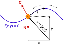
For a wide variety of physical systems, if the size and shape of a massive object are negligible, it is a useful simplification to treat it as a point particle. For a system of N point particles with masses m1, m2, ..., mN, each particle has a position vector, denoted r1, r2, ..., rN. Cartesian coordinates are often sufficient, so r1 = (x1, y1, z1), r2 = (x2, y2, z2) and so on. In three dimensional space, each position vector requires three coordinates to uniquely define the location of a point, so there are 3N coordinates to uniquely define the configuration of the system. These are all specific points in space to locate the particles; a general point in space is written r = (x, y, z). The velocity of each particle is how fast the particle moves along its path of motion, and is the time derivative of its position, thus


Lagrangian edit
Instead of forces, Lagrangian mechanics uses the energies in the system. The central quantity of Lagrangian mechanics is the Lagrangian, a function which summarizes the dynamics of the entire system. Overall, the Lagrangian has units of energy, but no single expression for all physical systems. Any function which generates the correct equations of motion, in agreement with physical laws, can be taken as a Lagrangian. It is nevertheless possible to construct general expressions for large classes of applications. The non-relativistic Lagrangian for a system of particles in the absence of an electromagnetic field is given by[5]


Kinetic energy is the energy of the system's motion, and vk2 = vk · vk is the magnitude squared of velocity, equivalent to the dot product of the velocity with itself. The kinetic energy is a function only of the velocities vk, not the positions rk nor time t, so T = T(v1, v2, ...).
The potential energy of the system reflects the energy of interaction between the particles, i.e. how much energy any one particle will have due to all the others and other external influences. For conservative forces (e.g. Newtonian gravity), it is a function of the position vectors of the particles only, so V = V(r1, r2, ...). For those non-conservative forces which can be derived from an appropriate potential (e.g. electromagnetic potential), the velocities will appear also, V = V(r1, r2, ..., v1, v2, ...). If there is some external field or external driving force changing with time, the potential will change with time, so most generally V = V(r1, r2, ..., v1, v2, ..., t).
The above form of L does not hold in relativistic Lagrangian mechanics or in the presence of a magnetic field when using the typical expression for the potential energy, and must be replaced by a function consistent with special or general relativity. Also, for dissipative forces (e.g., friction), another function must be introduced alongside L.
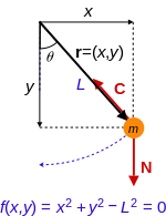
One or more of the particles may each be subject to one or more holonomic constraints; such a constraint is described by an equation of the form f(r, t) = 0. If the number of constraints in the system is C, then each constraint has an equation, f1(r, t) = 0, f2(r, t) = 0, ..., fC(r, t) = 0, each of which could apply to any of the particles. If particle k is subject to constraint i, then fi(rk, t) = 0. At any instant of time, the coordinates of a constrained particle are linked together and not independent. The constraint equations determine the allowed paths the particles can move along, but not where they are or how fast they go at every instant of time. Nonholonomic constraints depend on the particle velocities, accelerations, or higher derivatives of position. Lagrangian mechanics can only be applied to systems whose constraints, if any, are all holonomic. Three examples of nonholonomic constraints are:[7] when the constraint equations are nonintegrable, when the constraints have inequalities, or with complicated non-conservative forces like friction. Nonholonomic constraints require special treatment, and one may have to revert to Newtonian mechanics, or use other methods.
If T or V or both depend explicitly on time due to time-varying constraints or external influences, the Lagrangian L(r1, r2, ... v1, v2, ... t) is explicitly time-dependent. If neither the potential nor the kinetic energy depend on time, then the Lagrangian L(r1, r2, ... v1, v2, ...) is explicitly independent of time. In either case, the Lagrangian will always have implicit time-dependence through the generalized coordinates.
With these definitions, Lagrange's equations of the first kind are[8]

where k = 1, 2, ..., N labels the particles, there is a Lagrange multiplier λi for each constraint equation fi, and

In the Lagrangian, the position coordinates and velocity components are all independent variables, and derivatives of the Lagrangian are taken with respect to these separately according to the usual differentiation rules (e.g. the partial derivative of L with respect to the z-velocity component of particle 2, defined by vz,2 = dz2/dt, is just ∂L/∂vz,2; no awkward chain rules or total derivatives need to be used to relate the velocity component to the corresponding coordinate z2).
In each constraint equation, one coordinate is redundant because it is determined from the other coordinates. The number of independent coordinates is therefore n = 3N − C. We can transform each position vector to a common set of n generalized coordinates, conveniently written as an n-tuple q = (q1, q2, ... qn), by expressing each position vector, and hence the position coordinates, as functions of the generalized coordinates and time,

The vector q is a point in the configuration space of the system. The time derivatives of the generalized coordinates are called the generalized velocities, and for each particle the transformation of its velocity vector, the total derivative of its position with respect to time, is

Given this vk, the kinetic energy in generalized coordinates depends on the generalized velocities, generalized coordinates, and time if the position vectors depend explicitly on time due to time-varying constraints, so .

With these definitions, the Euler–Lagrange equations, or Lagrange's equations of the second kind[9][10]

are mathematical results from the calculus of variations, which can also be used in mechanics. Substituting in the Lagrangian L(q, dq/dt, t), gives the equations of motion of the system. The number of equations has decreased compared to Newtonian mechanics, from 3N to n = 3N − C coupled second order differential equations in the generalized coordinates. These equations do not include constraint forces at all, only non-constraint forces need to be accounted for.
Although the equations of motion include partial derivatives, the results of the partial derivatives are still ordinary differential equations in the position coordinates of the particles. The total time derivative denoted d/dt often involves implicit differentiation. Both equations are linear in the Lagrangian, but will generally be nonlinear coupled equations in the coordinates.
From Newtonian to Lagrangian mechanics edit
Newton's laws edit

For simplicity, Newton's laws can be illustrated for one particle without much loss of generality (for a system of N particles, all of these equations apply to each particle in the system). The equation of motion for a particle of constant mass m is Newton's second law of 1687, in modern vector notation

Newton's laws are easy to use in Cartesian coordinates, but Cartesian coordinates are not always convenient, and for other coordinate systems the equations of motion can become complicated. In a set of curvilinear coordinates ξ = (ξ1, ξ2, ξ3), the law in tensor index notation is the "Lagrangian form"[11][12]


It may seem like an overcomplication to cast Newton's law in this form, but there are advantages. The acceleration components in terms of the Christoffel symbols can be avoided by evaluating derivatives of the kinetic energy instead. If there is no resultant force acting on the particle, F = 0, it does not accelerate, but moves with constant velocity in a straight line. Mathematically, the solutions of the differential equation are geodesics, the curves of extremal length between two points in space (these may end up being minimal so the shortest paths, but that is not necessary). In flat 3D real space the geodesics are simply straight lines. So for a free particle, Newton's second law coincides with the geodesic equation, and states that free particles follow geodesics, the extremal trajectories it can move along. If the particle is subject to forces, F ≠ 0, the particle accelerates due to forces acting on it, and deviates away from the geodesics it would follow if free. With appropriate extensions of the quantities given here in flat 3D space to 4D curved spacetime, the above form of Newton's law also carries over to Einstein's general relativity, in which case free particles follow geodesics in curved spacetime that are no longer "straight lines" in the ordinary sense.[13]
However, we still need to know the total resultant force F acting on the particle, which in turn requires the resultant non-constraint force N plus the resultant constraint force C,

The constraint forces can be complicated, since they will generally depend on time. Also, if there are constraints, the curvilinear coordinates are not independent but related by one or more constraint equations.
The constraint forces can either be eliminated from the equations of motion so only the non-constraint forces remain, or included by including the constraint equations in the equations of motion.
D'Alembert's principle edit

A fundamental result in analytical mechanics is D'Alembert's principle, introduced in 1708 by Jacques Bernoulli to understand static equilibrium, and developed by D'Alembert in 1743 to solve dynamical problems.[14] The principle asserts for N particles the virtual work, i.e. the work along a virtual displacement, δrk, is zero:[6]

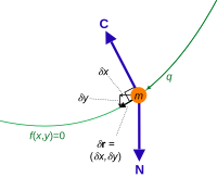
The virtual displacements, δrk, are by definition infinitesimal changes in the configuration of the system consistent with the constraint forces acting on the system at an instant of time,[15] i.e. in such a way that the constraint forces maintain the constrained motion. They are not the same as the actual displacements in the system, which are caused by the resultant constraint and non-constraint forces acting on the particle to accelerate and move it.[nb 2] Virtual work is the work done along a virtual displacement for any force (constraint or non-constraint).
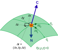
Since the constraint forces act perpendicular to the motion of each particle in the system to maintain the constraints, the total virtual work by the constraint forces acting on the system is zero:[16][nb 3]


Thus D'Alembert's principle allows us to concentrate on only the applied non-constraint forces, and exclude the constraint forces in the equations of motion.[17][18] The form shown is also independent of the choice of coordinates. However, it cannot be readily used to set up the equations of motion in an arbitrary coordinate system since the displacements δrk might be connected by a constraint equation, which prevents us from setting the N individual summands to 0. We will therefore seek a system of mutually independent coordinates for which the total sum will be 0 if and only if the individual summands are 0. Setting each of the summands to 0 will eventually give us our separated equations of motion.
Equations of motion from D'Alembert's principle edit
If there are constraints on particle k, then since the coordinates of the position rk = (xk, yk, zk) are linked together by a constraint equation, so are those of the virtual displacements δrk = (δxk, δyk, δzk). Since the generalized coordinates are independent, we can avoid the complications with the δrk by converting to virtual displacements in the generalized coordinates. These are related in the same form as a total differential,[6]

There is no partial time derivative with respect to time multiplied by a time increment, since this is a virtual displacement, one along the constraints in an instant of time.
The first term in D'Alembert's principle above is the virtual work done by the non-constraint forces Nk along the virtual displacements δrk, and can without loss of generality be converted into the generalized analogues by the definition of generalized forces


This is half of the conversion to generalized coordinates. It remains to convert the acceleration term into generalized coordinates, which is not immediately obvious. Recalling the Lagrange form of Newton's second law, the partial derivatives of the kinetic energy with respect to the generalized coordinates and velocities can be found to give the desired result:[6]

Now D'Alembert's principle is in the generalized coordinates as required,
![{\displaystyle \sum _{j=1}^{n}\left[Q_{j}-\left({\frac {\mathrm {d} }{\mathrm {d} t}}{\frac {\partial T}{\partial {\dot {q}}_{j}}}-{\frac {\partial T}{\partial q_{j}}}\right)\right]\delta q_{j}=0\,,}](https://wikimedia.org/api/rest_v1/media/math/render/svg/cf81ebf14cb6b43779228e274d39444e1a4d7787)

These equations are equivalent to Newton's laws for the non-constraint forces. The generalized forces in this equation are derived from the non-constraint forces only – the constraint forces have been excluded from D'Alembert's principle and do not need to be found. The generalized forces may be non-conservative, provided they satisfy D'Alembert's principle.[22]
Euler–Lagrange equations and Hamilton's principle edit
For a non-conservative force which depends on velocity, it may be possible to find a potential energy function V that depends on positions and velocities. If the generalized forces Qi can be derived from a potential V such that[24][25]


However, the Euler–Lagrange equations can only account for non-conservative forces if a potential can be found as shown. This may not always be possible for non-conservative forces, and Lagrange's equations do not involve any potential, only generalized forces; therefore they are more general than the Euler–Lagrange equations.
The Euler–Lagrange equations also follow from the calculus of variations. The variation of the Lagrangian is

![{\displaystyle \int _{t_{1}}^{t_{2}}\delta L\,\mathrm {d} t=\int _{t_{1}}^{t_{2}}\sum _{j=1}^{n}\left({\frac {\partial L}{\partial q_{j}}}\delta q_{j}+{\frac {\mathrm {d} }{\mathrm {d} t}}\left({\frac {\partial L}{\partial {\dot {q}}_{j}}}\delta q_{j}\right)-{\frac {\mathrm {d} }{\mathrm {d} t}}{\frac {\partial L}{\partial {\dot {q}}_{j}}}\delta q_{j}\right)\,\mathrm {d} t\,=\sum _{j=1}^{n}\left[{\frac {\partial L}{\partial {\dot {q}}_{j}}}\delta q_{j}\right]_{t_{1}}^{t_{2}}+\int _{t_{1}}^{t_{2}}\sum _{j=1}^{n}\left({\frac {\partial L}{\partial q_{j}}}-{\frac {\mathrm {d} }{\mathrm {d} t}}{\frac {\partial L}{\partial {\dot {q}}_{j}}}\right)\delta q_{j}\,\mathrm {d} t\,.}](https://wikimedia.org/api/rest_v1/media/math/render/svg/54a48053647f191bd378c62f02e1dc5e53fdfb4e)
Now, if the condition δqj(t1) = δqj(t2) = 0 holds for all j, the terms not integrated are zero. If in addition the entire time integral of δL is zero, then because the δqj are independent, and the only way for a definite integral to be zero is if the integrand equals zero, each of the coefficients of δqj must also be zero. Then we obtain the equations of motion. This can be summarized by Hamilton's principle:

The time integral of the Lagrangian is another quantity called the action, defined as[26]


Thus, instead of thinking about particles accelerating in response to applied forces, one might think of them picking out the path with a stationary action, with the end points of the path in configuration space held fixed at the initial and final times. Hamilton's principle is sometimes referred to as the principle of least action, however the action functional need only be stationary, not necessarily a maximum or a minimum value. Any variation of the functional gives an increase in the functional integral of the action.
Historically, the idea of finding the shortest path a particle can follow subject to a force motivated the first applications of the calculus of variations to mechanical problems, such as the Brachistochrone problem solved by Jean Bernoulli in 1696, as well as Leibniz, Daniel Bernoulli, L'Hôpital around the same time, and Newton the following year.[27] Newton himself was thinking along the lines of the variational calculus, but did not publish.[27] These ideas in turn lead to the variational principles of mechanics, of Fermat, Maupertuis, Euler, Hamilton, and others.
Hamilton's principle can be applied to nonholonomic constraints if the constraint equations can be put into a certain form, a linear combination of first order differentials in the coordinates. The resulting constraint equation can be rearranged into first order differential equation.[28] This will not be given here.
Lagrange multipliers and constraints edit
The Lagrangian L can be varied in the Cartesian rk coordinates, for N particles,

Hamilton's principle is still valid even if the coordinates L is expressed in are not independent, here rk, but the constraints are still assumed to be holonomic.[29] As always the end points are fixed δrk(t1) = δrk(t2) = 0 for all k. What cannot be done is to simply equate the coefficients of δrk to zero because the δrk are not independent. Instead, the method of Lagrange multipliers can be used to include the constraints. Multiplying each constraint equation fi(rk, t) = 0 by a Lagrange multiplier λi for i = 1, 2, ..., C, and adding the results to the original Lagrangian, gives the new Lagrangian

The Lagrange multipliers are arbitrary functions of time t, but not functions of the coordinates rk, so the multipliers are on equal footing with the position coordinates. Varying this new Lagrangian and integrating with respect to time gives

The introduced multipliers can be found so that the coefficients of δrk are zero, even though the rk are not independent. The equations of motion follow. From the preceding analysis, obtaining the solution to this integral is equivalent to the statement


For the case of a conservative force given by the gradient of some potential energy V, a function of the rk coordinates only, substituting the Lagrangian L = T − V gives


Properties of the Lagrangian edit
Non-uniqueness edit
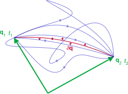
The Lagrangian of a given system is not unique. A Lagrangian L can be multiplied by a nonzero constant a and shifted by an arbitrary constant b, and the new Lagrangian L′ = aL + b will describe the same motion as L. If one restricts as above to trajectories q over a given time interval [tst, tfin]} and fixed end points Pst = q(tst) and Pfin = q(tfin), then two Lagrangians describing the same system can differ by the "total time derivative" of a function f(q, t):[30]


Both Lagrangians L and L′ produce the same equations of motion[31][32] since the corresponding actions S and S′ are related via
![{\displaystyle {\begin{aligned}S'[\mathbf {q} ]&=\int _{t_{\text{st}}}^{t_{\text{fin}}}L'(\mathbf {q} (t),{\dot {\mathbf {q} }}(t),t)\,dt\\[1ex]&=\int _{t_{\text{st}}}^{t_{\text{fin}}}L(\mathbf {q} (t),{\dot {\mathbf {q} }}(t),t)\,dt+\int _{t_{\text{st}}}^{t_{\text{fin}}}{\frac {\mathrm {d} f(\mathbf {q} (t),t)}{\mathrm {d} t}}\,dt\\[1ex]&=S[\mathbf {q} ]+f(P_{\text{fin}},t_{\text{fin}})-f(P_{\text{st}},t_{\text{st}}),\end{aligned}}}](https://wikimedia.org/api/rest_v1/media/math/render/svg/ef9eeb77d9dd2e4400201c2a835fc20a768980ff)
Invariance under point transformations edit
Given a set of generalized coordinates q, if we change these variables to a new set of generalized coordinates Q according to a point transformation Q = Q(q, t) which is invertible as q = q(Q, t), the new Lagrangian L′ is a function of the new coordinates


This may simplify the equations of motion.
For a coordinate transformation , we have


It also follows that:


Starting from Euler Lagrange equations in initial set of generalized coordinates, we have:

Since the transformation from is invertible, it follows that the form of the Euler-Lagrange equation is invariant i.e.,


Cyclic coordinates and conserved momenta edit
An important property of the Lagrangian is that conserved quantities can easily be read off from it. The generalized momentum "canonically conjugate to" the coordinate qi is defined by

If the Lagrangian L does not depend on some coordinate qi, it follows immediately from the Euler–Lagrange equations that

For example, a system may have a Lagrangian


Energy edit
Given a Lagrangian the Hamiltonian of the corresponding mechanical system is, by definition,


Invariance under coordinate transformations edit
At every time instant t, the energy is invariant under configuration space coordinate changes q → Q, i.e. (using natural coordinates)


For a coordinate transformation Q = F(q), we have


In vector notation,

On the other hand,

It was mentioned earlier that Lagrangians do not depend on the choice of configuration space coordinates, i.e. One implication of this is that and


Conservation edit
In Lagrangian mechanics, the system is closed if and only if its Lagrangian does not explicitly depend on time. The energy conservation law states that the energy of a closed system is an integral of motion.

More precisely, let q = q(t) be an extremal. (In other words, q satisfies the Euler–Lagrange equations). Taking the total time-derivative of L along this extremal and using the EL equations leads to

If the Lagrangian L does not explicitly depend on time, then ∂L/∂t = 0, then H does not vary with time evolution of particle, indeed, an integral of motion, meaning that

Kinetic and potential energies edit
Under all these circumstances,[34] the constant

Mechanical similarity edit
If the potential energy is a homogeneous function of the coordinates and independent of time,[35] and all position vectors are scaled by the same nonzero constant α, rk′ = αrk, so that


Since the lengths and times have been scaled, the trajectories of the particles in the system follow geometrically similar paths differing in size. The length l traversed in time t in the original trajectory corresponds to a new length l′ traversed in time t′ in the new trajectory, given by the ratios

Interacting particles edit
For a given system, if two subsystems A and B are non-interacting, the Lagrangian L of the overall system is the sum of the Lagrangians LA and LB for the subsystems:[30]

If they do interact this is not possible. In some situations, it may be possible to separate the Lagrangian of the system L into the sum of non-interacting Lagrangians, plus another Lagrangian LAB containing information about the interaction,

This may be physically motivated by taking the non-interacting Lagrangians to be kinetic energies only, while the interaction Lagrangian is the system's total potential energy. Also, in the limiting case of negligible interaction, LAB tends to zero reducing to the non-interacting case above.
The extension to more than two non-interacting subsystems is straightforward – the overall Lagrangian is the sum of the separate Lagrangians for each subsystem. If there are interactions, then interaction Lagrangians may be added.
Consequences of singular Lagrangians edit
From the Euler-Lagrange equations, it follows that:

Where the matrix is defined as . If the matrix is non-singular, the above equations can be solved to represent as a function of . If the matrix is non-invertible, it would not be possible to represent all 's as a function of but also, the Hamiltonian equations of motions will not take the standard form.[36]


Examples edit
The following examples apply Lagrange's equations of the second kind to mechanical problems.
Conservative force edit
A particle of mass m moves under the influence of a conservative force derived from the gradient ∇ of a scalar potential,

If there are more particles, in accordance with the above results, the total kinetic energy is a sum over all the particle kinetic energies, and the potential is a function of all the coordinates.
Cartesian coordinates edit
The Lagrangian of the particle can be written

The equations of motion for the particle are found by applying the Euler–Lagrange equation, for the x coordinate


Polar coordinates in 2D and 3D edit
Using the spherical coordinates (r, θ, φ) as commonly used in physics (ISO 80000-2:2019 convention), where r is the radial distance to origin, θ is polar angle (also known as colatitude, zenith angle, normal angle, or inclination angle), and φ is the azimuthal angle, the Lagrangian for a central potential is


The Lagrangian in two-dimensional polar coordinates is recovered by fixing θ to the constant value π/2.
Pendulum on a movable support edit
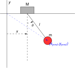
Consider a pendulum of mass m and length ℓ, which is attached to a support with mass M, which can move along a line in the -direction. Let be the coordinate along the line of the support, and let us denote the position of the pendulum by the angle from the vertical. The coordinates and velocity components of the pendulum bob are


The generalized coordinates can be taken to be and . The kinetic energy of the system is then


![{\displaystyle {\begin{array}{rcl}L&=&T-V\\&=&{\frac {1}{2}}M{\dot {x}}^{2}+{\frac {1}{2}}m\left[\left({\dot {x}}+\ell {\dot {\theta }}\cos \theta \right)^{2}+\left(\ell {\dot {\theta }}\sin \theta \right)^{2}\right]+mg\ell \cos \theta \\&=&{\frac {1}{2}}\left(M+m\right){\dot {x}}^{2}+m{\dot {x}}\ell {\dot {\theta }}\cos \theta +{\frac {1}{2}}m\ell ^{2}{\dot {\theta }}^{2}+mg\ell \cos \theta \,.\end{array}}}](https://wikimedia.org/api/rest_v1/media/math/render/svg/fcea9ca5dd9452880b94f4315f2430d4f9c88684)
Since x is absent from the Lagrangian, it is a cyclic coordinate. The conserved momentum is


The Lagrange equation for the angle θ is
![{\displaystyle {\frac {\mathrm {d} }{\mathrm {d} t}}\left[m({\dot {x}}\ell \cos \theta +\ell ^{2}{\dot {\theta }})\right]+m\ell ({\dot {x}}{\dot {\theta }}+g)\sin \theta =0;}](https://wikimedia.org/api/rest_v1/media/math/render/svg/27ef95240aa335e09f85c8c7ef67a7301547c588)

These equations may look quite complicated, but finding them with Newton's laws would have required carefully identifying all forces, which would have been much more laborious and prone to errors. By considering limit cases, the correctness of this system can be verified: For example, should give the equations of motion for a simple pendulum that is at rest in some inertial frame, while should give the equations for a pendulum in a constantly accelerating system, etc. Furthermore, it is trivial to obtain the results numerically, given suitable starting conditions and a chosen time step, by stepping through the results iteratively.


Two-body central force problem edit
Two bodies of masses m1 and m2 with position vectors r1 and r2 are in orbit about each other due to an attractive central potential V. We may write down the Lagrangian in terms of the position coordinates as they are, but it is an established procedure to convert the two-body problem into a one-body problem as follows. Introduce the Jacobi coordinates; the separation of the bodies r = r2 − r1 and the location of the center of mass R = (m1r1 + m2r2)/(m1 + m2). The Lagrangian is then[37][38][nb 4]

The Euler–Lagrange equation for R is simply

Since the relative motion only depends on the magnitude of the separation, it is ideal to use polar coordinates (r, θ) and take r = |r|,


The radial coordinate r and angular velocity dθ/dt can vary with time, but only in such a way that ℓ is constant. The Lagrange equation for r is

This equation is identical to the radial equation obtained using Newton's laws in a co-rotating reference frame, that is, a frame rotating with the reduced mass so it appears stationary. Eliminating the angular velocity dθ/dt from this radial equation,[39]


Of course, if one remains entirely within the one-dimensional formulation, ℓ enters only as some imposed parameter of the external outward force, and its interpretation as angular momentum depends upon the more general two-dimensional problem from which the one-dimensional problem originated.
If one arrives at this equation using Newtonian mechanics in a co-rotating frame, the interpretation is evident as the centrifugal force in that frame due to the rotation of the frame itself. If one arrives at this equation directly by using the generalized coordinates (r, θ) and simply following the Lagrangian formulation without thinking about frames at all, the interpretation is that the centrifugal force is an outgrowth of using polar coordinates. As Hildebrand says:[40]
"Since such quantities are not true physical forces, they are often called inertia forces. Their presence or absence depends, not upon the particular problem at hand, but upon the coordinate system chosen." In particular, if Cartesian coordinates are chosen, the centrifugal force disappears, and the formulation involves only the central force itself, which provides the centripetal force for a curved motion.
This viewpoint, that fictitious forces originate in the choice of coordinates, often is expressed by users of the Lagrangian method. This view arises naturally in the Lagrangian approach, because the frame of reference is (possibly unconsciously) selected by the choice of coordinates. For example, see[41] for a comparison of Lagrangians in an inertial and in a noninertial frame of reference. See also the discussion of "total" and "updated" Lagrangian formulations in.[42] Unfortunately, this usage of "inertial force" conflicts with the Newtonian idea of an inertial force. In the Newtonian view, an inertial force originates in the acceleration of the frame of observation (the fact that it is not an inertial frame of reference), not in the choice of coordinate system. To keep matters clear, it is safest to refer to the Lagrangian inertial forces as generalized inertial forces, to distinguish them from the Newtonian vector inertial forces. That is, one should avoid following Hildebrand when he says (p. 155) "we deal always with generalized forces, velocities accelerations, and momenta. For brevity, the adjective "generalized" will be omitted frequently."
It is known that the Lagrangian of a system is not unique. Within the Lagrangian formalism the Newtonian fictitious forces can be identified by the existence of alternative Lagrangians in which the fictitious forces disappear, sometimes found by exploiting the symmetry of the system.[43]
Extensions to include non-conservative forces edit
Dissipative forces edit
Dissipation (i.e. non-conservative systems) can also be treated with an effective Lagrangian formulated by a certain doubling of the degrees of freedom.[44][45][46][47]
In a more general formulation, the forces could be both conservative and viscous. If an appropriate transformation can be found from the Fi, Rayleigh suggests using a dissipation function, D, of the following form:[48]


Electromagnetism edit
A test particle is a particle whose mass and charge are assumed to be so small that its effect on external system is insignificant. It is often a hypothetical simplified point particle with no properties other than mass and charge. Real particles like electrons and up quarks are more complex and have additional terms in their Lagrangians. Not only can the fields form non conservative potentials, these potentials can also be velocity dependent.
The Lagrangian for a charged particle with electrical charge q, interacting with an electromagnetic field, is the prototypical example of a velocity-dependent potential. The electric scalar potential ϕ = ϕ(r, t) and magnetic vector potential A = A(r, t) are defined from the electric field E = E(r, t) and magnetic field B = B(r, t) as follows:

The Lagrangian of a massive charged test particle in an electromagnetic field


Under gauge transformation:


Note that the canonical momentum (conjugate to position r) is the kinetic momentum plus a contribution from the A field (known as the potential momentum):

This relation is also used in the minimal coupling prescription in quantum mechanics and quantum field theory. From this expression, we can see that the canonical momentum p is not gauge invariant, and therefore not a measurable physical quantity; However, if r is cyclic (i.e. Lagrangian is independent of position r), which happens if the ϕ and A fields are uniform, then this canonical momentum p given here is the conserved momentum, while the measurable physical kinetic momentum mv is not.
Other contexts and formulations edit
The ideas in Lagrangian mechanics have numerous applications in other areas of physics, and can adopt generalized results from the calculus of variations.
Alternative formulations of classical mechanics edit
A closely related formulation of classical mechanics is Hamiltonian mechanics. The Hamiltonian is defined by

Routhian mechanics is a hybrid formulation of Lagrangian and Hamiltonian mechanics, which is not often used in practice but an efficient formulation for cyclic coordinates.
Momentum space formulation edit
The Euler–Lagrange equations can also be formulated in terms of the generalized momenta rather than generalized coordinates. Performing a Legendre transformation on the generalized coordinate Lagrangian L(q, dq/dt, t) obtains the generalized momenta Lagrangian L′(p, dp/dt, t) in terms of the original Lagrangian, as well the EL equations in terms of the generalized momenta. Both Lagrangians contain the same information, and either can be used to solve for the motion of the system. In practice generalized coordinates are more convenient to use and interpret than generalized momenta.
Higher derivatives of generalized coordinates edit
There is no mathematical reason to restrict the derivatives of generalized coordinates to first order only. It is possible to derive modified EL equations for a Lagrangian containing higher order derivatives, see Euler–Lagrange equation for details. However, from the physical point-of-view there is an obstacle to include time derivatives higher than the first order, which is implied by Ostrogradsky's construction of a canonical formalism for nondegenerate higher derivative Lagrangians, see Ostrogradsky instability
Optics edit
Lagrangian mechanics can be applied to geometrical optics, by applying variational principles to rays of light in a medium, and solving the EL equations gives the equations of the paths the light rays follow.
Relativistic formulation edit
Lagrangian mechanics can be formulated in special relativity and general relativity. Some features of Lagrangian mechanics are retained in the relativistic theories but difficulties quickly appear in other respects. In particular, the EL equations take the same form, and the connection between cyclic coordinates and conserved momenta still applies, however the Lagrangian must be modified and is not simply the kinetic minus the potential energy of a particle. Also, it is not straightforward to handle multiparticle systems in a manifestly covariant way, it may be possible if a particular frame of reference is singled out.
Quantum mechanics edit
In quantum mechanics, action and quantum-mechanical phase are related via the Planck constant, and the principle of stationary action can be understood in terms of constructive interference of wave functions.
In 1948, Feynman discovered the path integral formulation extending the principle of least action to quantum mechanics for electrons and photons. In this formulation, particles travel every possible path between the initial and final states; the probability of a specific final state is obtained by summing over all possible trajectories leading to it. In the classical regime, the path integral formulation cleanly reproduces Hamilton's principle, and Fermat's principle in optics.
Classical field theory edit
In Lagrangian mechanics, the generalized coordinates form a discrete set of variables that define the configuration of a system. In classical field theory, the physical system is not a set of discrete particles, but rather a continuous field ϕ(r, t) defined over a region of 3D space. Associated with the field is a Lagrangian density


Noether's theorem edit
The action principle, and the Lagrangian formalism, are tied closely to Noether's theorem, which connects physical conserved quantities to continuous symmetries of a physical system.
If the Lagrangian is invariant under a symmetry, then the resulting equations of motion are also invariant under that symmetry. This characteristic is very helpful in showing that theories are consistent with either special relativity or general relativity.
See also edit
- Canonical coordinates
- Fundamental lemma of the calculus of variations
- Functional derivative
- Generalized coordinates
- Hamiltonian mechanics
- Hamiltonian optics
- Inverse problem for Lagrangian mechanics, the general topic of finding a Lagrangian for a system given the equations of motion.
- Lagrangian and Eulerian specification of the flow field
- Lagrangian point
- Lagrangian system
- Non-autonomous mechanics
- Plateau's problem
- Restricted three-body problem
Footnotes edit
- ^ Sometimes in this context the variational derivative denoted and defined as
is used. Throughout this article only partial and total derivatives are used.
- ^ Here the virtual displacements are assumed reversible, it is possible for some systems to have non-reversible virtual displacements that violate this principle, see Udwadia–Kalaba equation.
- ^ In other words
for particle k subject to a constraint force, howeverbecause of the constraint equations on the rk coordinates.
- ^ The Lagrangian also can be written explicitly for a rotating frame. See Padmanabhan, 2000.


Notes edit
- ^ Fraser, Craig. "J. L. Lagrange's Early Contributions to the Principles and Methods of Mechanics". Archive for History of Exact Sciences, vol. 28, no. 3, 1983, pp. 197–241. JSTOR, http://www.jstor.org/stable/41133689. Accessed 3 Nov. 2023.
- ^ Hand & Finch 1998, p. 23
- ^ Hand & Finch 1998, pp. 18–20
- ^ Hand & Finch 1998, pp. 46, 51
- ^ Torby 1984, p. 270
- ^ a b c d Torby 1984, p. 269
- ^ Hand & Finch 1998, p. 36–40
- ^ Hand & Finch 1998, p. 60–61
- ^ Hand & Finch 1998, p. 19
- ^ Penrose 2007
- ^ Kay 1988, p. 156
- ^ Synge & Schild 1949, p. 150–152
- ^ Foster & Nightingale 1995, p. 89
- ^ Hand & Finch 1998, p. 4
- ^ Goldstein 1980, pp. 16–18
- ^ Hand & Finch 1998, p. 15
- ^ Hand & Finch 1998, p. 15
- ^ Fetter & Walecka 1980, p. 53
- ^ Kibble & Berkshire 2004, p. 234
- ^ Fetter & Walecka 1980, p. 56
- ^ Hand & Finch 1998, p. 17
- ^ Hand & Finch 1998, p. 15–17
- ^ R. Penrose (2007). The Road to Reality. Vintage books. p. 474. ISBN 978-0-679-77631-4.
- ^ Goldstein 1980, p. 23
- ^ Kibble & Berkshire 2004, p. 234–235
- ^ Hand & Finch 1998, p. 51
- ^ a b Hand & Finch 1998, p. 44–45
- ^ Goldstein 1980
- ^ Fetter & Walecka 1980, pp. 68–70
- ^ a b Landau & Lifshitz 1976, p. 4
- ^ Goldstein, Poole & Safko 2002, p. 21
- ^ Landau & Lifshitz 1976, p. 4
- ^ Goldstein 1980, p. 21
- ^ Landau & Lifshitz 1976, p. 14
- ^ Landau & Lifshitz 1976, p. 22
- ^ Rothe, Heinz J; Rothe, Klaus D (2010). Classical and Quantum Dynamics of Constrained Hamiltonian Systems. World Scientific Lecture Notes in Physics. Vol. 81. WORLD SCIENTIFIC. p. 7. doi:10.1142/7689. ISBN 978-981-4299-64-0.
- ^ Taylor 2005, p. 297
- ^ Padmanabhan 2000, p. 48
- ^ Hand & Finch 1998, pp. 140–141
- ^ Hildebrand 1992, p. 156
- ^ Zak, Zbilut & Meyers 1997, pp. 202
- ^ Shabana 2008, pp. 118–119
- ^ Gannon 2006, p. 267
- ^ Kosyakov 2007
- ^ Galley 2013
- ^ Birnholtz, Hadar & Kol 2014
- ^ Birnholtz, Hadar & Kol 2013
- ^ a b Torby 1984, p. 271
References edit
- Lagrange, J. L. (1811). Mécanique analytique. Vol. 1.
- Lagrange, J. L. (1815). Mécanique analytique. Vol. 2.
- Penrose, Roger (2007). The Road to Reality. Vintage books. ISBN 978-0-679-77631-4.
- Landau, L. D.; Lifshitz, E. M. (15 January 1976). Mechanics (3rd ed.). Butterworth Heinemann. p. 134. ISBN 9780750628969.
- Landau, Lev; Lifshitz, Evgeny (1975). The Classical Theory of Fields. Elsevier Ltd. ISBN 978-0-7506-2768-9.
- Hand, L. N.; Finch, J. D. (1998). Analytical Mechanics (2nd ed.). Cambridge University Press. ISBN 9780521575720.
- Saletan, E. J.; José, J. V. (1998). Classical Dynamics: A Contemporary Approach. Cambridge University Press. ISBN 9780521636360.
- Kibble, T. W. B.; Berkshire, F. H. (2004). Classical Mechanics (5th ed.). Imperial College Press. p. 236. ISBN 9781860944352.
- Goldstein, Herbert (1980). Classical Mechanics (2nd ed.). San Francisco, CA: Addison Wesley. ISBN 0201029189.
- Goldstein, Herbert; Poole, Charles P. Jr.; Safko, John L. (2002). Classical Mechanics (3rd ed.). San Francisco, CA: Addison Wesley. ISBN 0-201-65702-3.
- Lanczos, Cornelius (1986). "II §5 Auxiliary conditions: the Lagrangian λ-method". The variational principles of mechanics (Reprint of University of Toronto 1970 4th ed.). Courier Dover. p. 43. ISBN 0-486-65067-7.
- Fetter, A. L.; Walecka, J. D. (1980). Theoretical Mechanics of Particles and Continua. Dover. pp. 53–57. ISBN 978-0-486-43261-8.
- The Principle of Least Action, R. Feynman
- Dvorak, R.; Freistetter, Florian (2005). "§ 3.2 Lagrange equations of the first kind". Chaos and stability in planetary systems. Birkhäuser. p. 24. ISBN 3-540-28208-4.
- Haken, H (2006). Information and self-organization (3rd ed.). Springer. p. 61. ISBN 3-540-33021-6.
- Henry Zatzkis (1960). "§1.4 Lagrange equations of the second kind". In DH Menzel (ed.). Fundamental formulas of physics. Vol. 1 (2nd ed.). Courier Dover. p. 160. ISBN 0-486-60595-7.
- Hildebrand, Francis Begnaud (1992). Methods of applied mathematics (Reprint of Prentice-Hall 1965 2nd ed.). Courier Dover. p. 156. ISBN 0-486-67002-3.
- Zak, Michail; Zbilut, Joseph P.; Meyers, Ronald E. (1997). From instability to intelligence. Springer. p. 202. ISBN 3-540-63055-4.
- Shabana, Ahmed A. (2008). Computational continuum mechanics. Cambridge University Press. pp. 118–119. ISBN 978-0-521-88569-0.
- Taylor, John Robert (2005). Classical mechanics. University Science Books. p. 297. ISBN 1-891389-22-X.
- Padmanabhan, Thanu (2000). "§2.3.2 Motion in a rotating frame". Theoretical Astrophysics: Astrophysical processes (3rd ed.). Cambridge University Press. p. 48. ISBN 0-521-56632-0.
- Doughty, Noel A. (1990). Lagrangian Interaction. Addison-Wesley Publishers Ltd. ISBN 0-201-41625-5.
- Kosyakov, B. P. (2007). Introduction to the classical theory of particles and fields. Berlin, Germany: Springer. doi:10.1007/978-3-540-40934-2. ISBN 978-3-540-40933-5.
- Galley, Chad R. (2013). "Classical Mechanics of Nonconservative Systems". Physical Review Letters. 110 (17): 174301. arXiv:1210.2745. Bibcode:2013PhRvL.110q4301G. doi:10.1103/PhysRevLett.110.174301. PMID 23679733. S2CID 14591873.
- Birnholtz, Ofek; Hadar, Shahar; Kol, Barak (2014). "Radiation reaction at the level of the action". International Journal of Modern Physics A. 29 (24): 1450132–1450190. arXiv:1402.2610. Bibcode:2014IJMPA..2950132B. doi:10.1142/S0217751X14501322. S2CID 118541484.
- Birnholtz, Ofek; Hadar, Shahar; Kol, Barak (2013). "Theory of post-Newtonian radiation and reaction". Physical Review D. 88 (10): 104037. arXiv:1305.6930. Bibcode:2013PhRvD..88j4037B. doi:10.1103/PhysRevD.88.104037. S2CID 119170985.
- Roger F Gans (2013). Engineering Dynamics: From the Lagrangian to Simulation. New York: Springer. ISBN 978-1-4614-3929-5.
- Gannon, Terry (2006). Moonshine beyond the monster: the bridge connecting algebra, modular forms and physics. Cambridge University Press. p. 267. ISBN 0-521-83531-3.
- Torby, Bruce (1984). "Energy Methods". Advanced Dynamics for Engineers. HRW Series in Mechanical Engineering. United States of America: CBS College Publishing. ISBN 0-03-063366-4.
- Foster, J; Nightingale, J.D. (1995). A Short Course in General Relativity (2nd ed.). Springer. ISBN 0-03-063366-4.
- M. P. Hobson; G. P. Efstathiou; A. N. Lasenby (2006). General Relativity: An Introduction for Physicists. Cambridge University Press. pp. 79–80. ISBN 9780521829519.
- Synge, J.L.; Schild, A. (1949). Tensor Calculus. first Dover Publications 1978 edition. ISBN 978-0-486-63612-2.
- Kay, David (April 1988). Schaum's Outline of Tensor Calculus. McGraw Hill Professional. ISBN 978-0-07-033484-7.
Further reading edit
- Gupta, Kiran Chandra, Classical mechanics of particles and rigid bodies (Wiley, 1988).
- Cassel, Kevin (2013). Variational methods with applications in science and engineering. Cambridge: Cambridge University Press. ISBN 978-1-107-02258-4.
- Goldstein, Herbert, et al. Classical Mechanics. 3rd ed., Pearson, 2002.
External links edit
- David Tong. "Cambridge Lecture Notes on Classical Dynamics". DAMTP. Retrieved 2017-06-08.
- Principle of least action interactive Excellent interactive explanation/webpage
- Joseph Louis de Lagrange - Œuvres complètes (Gallica-Math)
- Constrained motion and generalized coordinates, page 4